
Heuristic Optimal Meeting Point Algorithm for Car-Sharing in Large
Multimodal Road Networks
Julien Baudru
1,2 a
and Hugues Bersini
1,2 b
1
IRIDIA, Universit
´
e Libre de Bruxelles (ULB), Brussels, Belgium
2
FARI, AI for the Common Good Institute, Brussels, Belgium
Keywords:
Car-Pooling, Car-Sharing, Sustainable Mobility, Smart Transportation, Multimodal Networks & Road
Networks.
Abstract:
This article introduces a new version of the car-pooling problem (CPP). This involves defining rendezvous or
meeting point in such a way that the travel times of the users are fair, this problem shares similarities with the
problem of finding the optimal meeting point (OMP) in a graph. We propose a heuristic algorithm to solve the
OMP problem in this new context and compare its results with those of the exact solution algorithm, showing
its low error rate and short runtime. Finally, we propose some exploratory directions for future research.
1 INTRODUCTION
For several decades, the use of private vehicles has
exploded, leading to an increase in traffic congestion,
pollution, and accidents. Various solutions already
exist, such as public transport, however, since not
all cities have a well-developed public transport
network, car-sharing seems to be the most viable
alternative for users in terms of economy, ecology,
and comfort (Yu et al., 2017). Car-pooling can be
described as a shared transport system in which
users take a common route and therefore vehicle
to reach their different, or common, destinations.
This transport system is based on the shared use
of private vehicles. However, the primary aim of
existing car-pooling solutions is to be profitable,
either for the companies offering this services or for
the private drivers, which raises the question of fair
car-pooling. In the particular context of universities,
solving this challenge becomes important not only for
the reasons listed above but also because according
to (Lu
`
e and Colorni, 2009) around 78% of students
travel alone by car. In addition, according to (G
¨
arling
et al., 2000), the propensity to practice peer-to-peer
car-pooling is higher among younger people. Given
that this research is ultimately intended to be offered
as an application to students at the Universit
´
e Libre
de Bruxelles (ULB), the aforementioned arguments
a
https://orcid.org/0000-0002-8771-2494
b
https://orcid.org/0000-0001-5820-7360
strongly support the usefulness and potential of our
work. In the literature, the principal subject related
to car-pooling dealt with the matching of users, in
this field a distinction is commonly made between
two categories of car-pooling problems. The first,
known as the Daily Car Pooling Problem (DCPP),
aims to assign pedestrians to drivers and define the
routes they will take, while minimizing total travel
costs and respecting the constraints of time and
seats available in the car. The DCPP problem is
known as NP-hard since this is a particular case of
the Vehicle Routing Problem (VPR) which has been
proved NP-hard by (Toth et al., 2014). The second,
known as the Long Term Car Pooling Problem
(LTCPP), aims to create pools of users, knowing that
some users may be drivers one day and pedestrians
another, while maximizing the size of these pools,
minimizing the distance covered by the drivers and
respecting the same constraints as for the DCPP. In
addition, the Car-Pooling Problem (CPP) usually
falls into three types: 1) the many-to-one problem,
which requires moving from multiple origins to
a single destination, like the to-work problem; 2)
the one-to-many problem, which involves moving
from one origin to multiple destinations, like the
return-from-work problem; and 3) the many-to-many
problem, which involves moving from multiple
origins to multiple destinations, like the dial-a-ride
problem. It is important to point out that the dial-
a-ride problem differs from the CPP on the point of
vehicle ownership. In dial-a-ride, the driver serves
Baudru, J. and Bersini, H.
Heuristic Optimal Meeting Point Algorithm for Car-Sharing in Large Multimodal Road Networks.
DOI: 10.5220/0012719100003702
Paper published under CC license (CC BY-NC-ND 4.0)
In Proceedings of the 10th International Conference on Vehicle Technology and Intelligent Transport Systems (VEHITS 2024), pages 427-436
ISBN: 978-989-758-703-0; ISSN: 2184-495X
Proceedings Copyright © 2024 by SCITEPRESS – Science and Technology Publications, Lda.
427

the passengers full-time, whereas, in CPP, the vehicle
belongs to the participants, who can either act as
drivers or passengers. Furthermore, the car-sharing
problem addressed in this article does not take the
form of station-based but rather of free-floating.
However, as the authors of (Gedam, Celesty et al.,
2020) points out, in the majority of car-pooling sys-
tems proposed today, DCPP or LTCPP, users have to
explicitly specify the pickup and drop locations. The
solution proposed in this article solves this problem
by automatically generating a meeting point that is
fair to all users. This problem can be formulated
as follows: Given the presence of a walker and a
driver, what are the shortest paths to reach a meet-
ing point so that the travel times of each user are bal-
anced before reaching their common destination by
car? The meeting point M is described as the ren-
dezvous point between a driving user and a walking
user. The dropping point D, on the other hand, is de-
fined as the point where the driver drops a walking
user in order for both to continue their journeys to
their respective destinations. If we consider a simpler
case where the dropping D and destination points are
identical, the problem can be seen as a special case
of the many-to-one problem in car-pooling and this
problem can be called the search for the optimal meet-
ing point (OMP). However, the OMP problem usually
deals with distance, in these pages we’ll be looking
at a variant that focuses on travel time. The figure 1
illustrates the described problem. In this article, we
consider the case with identical dropping and desti-
nation points, and where we have only two users, a
driver and a walker. Note that the problem described
could be extended to several users of each type with
different destinations. In the remainder of this arti-
cle, we’ll assume that both users start their journeys
simultaneously. Finally, we introduce the use of mul-
timodal networks to the OMP search question. In fact,
in the model studied, two different transport networks
are considered, one for cars, and the other for pedes-
trians, each with their own specificities.
2 SIMILAR WORKS
In the following section, we delve into research on
car-pooling, optimal meeting points (OMP), and
road networks. This analysis contextualizes our
study within the existing literature, highlighting the
connections and distinctions between our research
and these crucial topics in transportation and urban
planning.
2.1 Car-Pooling
Concerning the particular context of shared cars be-
tween members of a university, which is also the
final applied purpose of this article, in (Bruglieri
et al., 2011) the authors propose a system called
PoliUniPool in which optimal groups of users within
the various universities of Milan are created using
a guided Monte Carlo simulation. However, this
system cannot provide users with real-time results
and requires prior offline calculation. In addition,
in (Laupichler and Sanders, 2023) the authors pro-
pose an algorithm called Karlsruhe Rapide Rideshar-
ing (KaRRi) for scheduling a fleet of shared vehi-
cles. The advantage of this solution is that it allows
the insertion of new passengers on existing routes.
This algorithm is based on the idea of the LOUD sys-
tem proposed by (Buchhold et al., 2021) using the
bucket contraction hierarchies (BCH) technique for
route networks to avoid a huge number of calls to the
Dijkstra algorithm. However, unlike our work, the
latter does not take into account the characteristics of
the road networks associated with the different modes
of transport. In addition, KaRRi has the particularity
of being able to handle numerous pickup and dropoff
points. Finally, the authors have shown that it is possi-
ble to reduce trip time and vehicle operating time by
extending car-sharing with walking. To our knowl-
edge, (Laupichler and Sanders, 2023) is one of the
few articles to address the multimodal aspect of the
road network in the context of car-sharing.
2.2 Optimal Meeting Point (OMP)
In (Huang et al., 2018), the authors model the prob-
lem of finding the optimal meeting point for two users
having their own source and destination points where
they need to meet before going to their destinations.
To do that they define a minimum path pair (MPP)
query, which consists of two pairs of source and des-
tination and a user-specified weight α to balance the
two different needs. The parameter α reflects the
need to go to the optimal meeting point (α ≥ 2) or
to go directly to the destination by the shortest path
(α=0). The weight α describes the requirement of
meeting. The larger α is, the stronger the demand
will be. Thanks to the α parameter, the authors intro-
duce the notion of certainty concerning the meeting
point, as in some cases the meeting is not possible or
beneficial for any user. Finally, they proposed an effi-
cient algorithm based on a point-to-point shortest path
and two fast approximate algorithms with approxima-
tion bounds. This point-to-point algorithm surpassed
the two-phase convex-hull-based pruning algorithm
VEHITS 2024 - 10th International Conference on Vehicle Technology and Intelligent Transport Systems
428
HullWindow (HW2) proposed by (Yan et al., 2011)
to compute the OMP. In (Li et al., 2016), the authors
proposed two novel parameterized solutions based on
dynamic programming (DP) to solve the problem of
optimal multi-meeting points in the context of car-
sharing for a group of users.
2.3 Road Networks
In (Xu and Jacobsen, 2010), the authors define three
types of proximity relations that induce location con-
straints to model continuous spatio-temporal queries
among sets of moving objects in road networks.
These distance computations are the max-pairwise-
distance, the min-sum-distance, and the min-max-
distance, some of them will be discussed later in the
section 6.1. The authors proposed a novel moving
object indexing technique that achieves good perfor-
mances on real-world data thanks to a partitioning
scheme for road networks. In (Wu et al., 2012), the
authors compare four state-of-the-art techniques to
find the shortest path in the context of road networks,
these techniques are: Spatially Induced Linkage Cog-
nizance (SILC), Path-Coherent Pairs Decomposition
(PCPD), Contraction Hierarchies (CH), and Transit
Node Routing (TNR). They conclude that CH was the
preferable choice when both space efficiency and time
efficiency are major concerns.
3 PROBLEM FORMULATION
Before considering the algorithm proposed, let us for-
mulate the problem in a simplified way. Thus we will
focus on a case with two users, a pedestrian and a
driver, sharing the same destination point. In this con-
figuration, we want to find the meeting point that min-
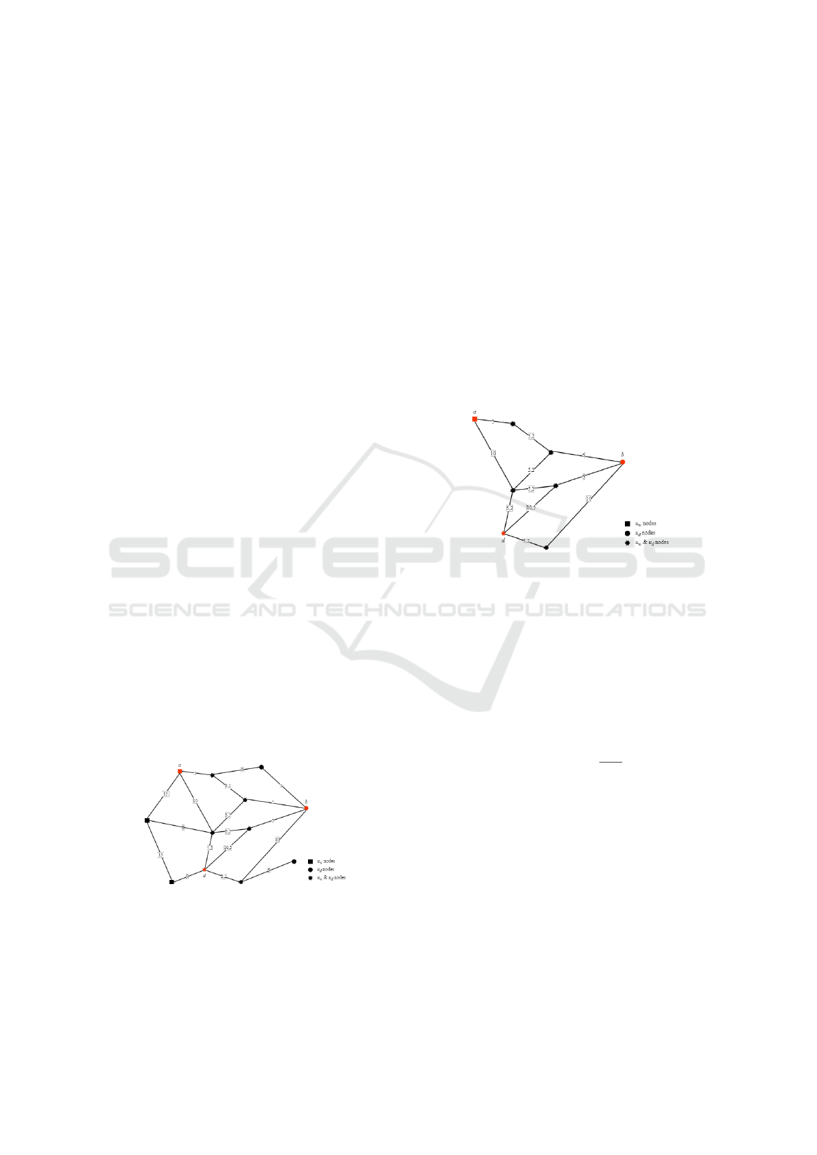
imizes the travel time for both users. Figure 1 illus-
trates this scenario.
Figure 1: G
w
& G
d
networks.
3.1 Optimal Meeting Point (OMP)
We define two directed weighted graphs, G
w
= {V,E}
the walking graph and G
d
= {V,E} the driving graph
representing the road networks for each user u, an
example is given in figure 1. Let a be the starting
point of the walking user u
w
, b the starting point
of the user u
d
and d the shared destination point of
u
w
and u
d
. Then, we define the directed weighted
graph G = {V,E} with V = {v
1
,v
2
,...,v
n
/v
i
∈ (G
w
∩
G
d
) ∪ (a, b)}, i.e. the set of road intersections com-
mon to G
w
and G
d
with the starting points of the
two users. The edges of G = {V, E} are defined as
E = {arc(i, j)/i ∈ V, j ∈ V }, i.e. the set of roads
between these intersections. An example of such a
graph is given in figure 2. Practical details of this op-
eration are given in section 5.1.
Figure 2: G network.
For each arc(i, j), a non-negative travel cost δ
i, j
is
associated, which corresponds to the distance of the
road between intersections i and j, each arc(i, j) also
have a travel speed σ
u
i, j
depending on the user u. We
denote by p
u
(i, j) the subset of V containing the se-
quence of nodes {v
1
,v
2
,..., v
n
} from the arcs included
in the path of user u to travel from the source i to the
destination j. We denoted by t
u
i, j
the travel time for
user u to complete path p
u
(i, j) such that:
t
u
i, j
=
∑
v,v
′
∈p
u
(i, j)
δ
v,v
′
σ
u
v,v
′
!
3.1.1 Objective Functions
Based on these definitions, we can establish several
objective functions. The two popular ways to define
the OMP are the min-max and the min-sub. For the
min-max, a first approach involves choosing m in such
a way as to minimize the travel time of each user like
in the Equation 2.
f = min
m
h
max
t
u
w
a,m
+t
u
d
m,d
, t
u
d
b,m
+t
u
d
m,d
i
(1)
= min
m
h
max
t
u
w
a,m
, t
u
d
b,m
i
(2)
Heuristic Optimal Meeting Point Algorithm for Car-Sharing in Large Multimodal Road Networks
429

A second approach involves choosing m in such
a way that it minimizes the travel time for each user
while ignoring the common path for the walker u
w
like in the Equation 3.
f = min
m
h
max
t
u
w
a,m
, t
u
d
b,m
+t
u
d
m,d
i
(3)
For the min-sub, a variant approach involves
choosing m in such a way that it minimizes the differ-
ence between the travel times to the meeting point m
for each user, i.e. their travel times must be as close
as possible. The waiting time t
wait
=
t
u
w
a,m
− t
u
d
b,m
at
the meeting point m is minimized by the Equation 4.
f = min
m
t
u
w
a,m
− t
u
d
b,m
(4)
3.2 Minimum Steiner Tree (MST)
This problem can also be seen as a variant of the min-
imum Steiner tree (MST) problem. For a set of nodes
W = {v
1
,v
2
,..., v
n
}, a subset of V , the Steiner tree
is a tree denoted S which spans all the nodes in W .
In the present case, W contains at least the source
nodes and the common destination node, such that
W = {a, b,d, ...,v
n
} and the meeting point m will be
one of the v
i
nodes in S. The travel time of S is given
by the Equation 5.
t
u
S
=
∑
v,v
′
∈S
δ
v,v
′
σ
u
v,v
′
!
(5)
The minimum Steiner tree is the Steiner tree with
the minimum travel time t
u
i, j
for each user u is denoted
by S∗. The MST is the S that minimizes the Equation
6.
f = min
S
t
u
S
(6)
3.3 Minimum Path Pair (MPP)
The minimum path pair (MPP) problem is to find
the path pair that minimizes a given function for two
pairs of source and destination, namely, (v
1
s
,v
1
t
) and
(v
2
s
,v
2
t
), with a parameter α. There are 3 costs: a) the
cost of the path of p
1
from v
1
s
to v
1
t
, b) the cost of
the path of p
2
from v
2
s
to v
2
t
, and c) the cost between
the two such paths p
1
and p
2
. Let w(p) be the cost
of a path p, and the distance between two paths, p1
and p2, be δ(p
1
, p
2
). The MPP is the pair of path to
minimize the Equation 7:
f = min
p
1
,p
2
w(p
1
) + w(p
2
) + δ(p
1
, p
2
) (7)
The path distance of a path p, w(p), is defined as
the sum of weights of its constituent edges:
w(p) =
∑
v,v
′
∈P
w(v,v
′
)
And the distance between the two paths p
1
and
p
2
, δ(p
1
, p
2
), is the shortest distance between a pair
of nodes, v
1
i
and v
2
j
:
δ(p
1
, p
2
) = min
v
1
i
∈p
1
,v
2
j
∈p
2
δ(v
1
i
,v
2
j
)
4 EXACT SOLUTION
In this section, we present two variations of the
algorithm for finding the OMP exactly, compare
the complexities of both algorithms, and detail their
operations.
To solve the problem of defining the rendezvous
point exactly, the OMP, one naive solution is to com-
pute the shortest path for each of the possible configu-
rations. Algorithm 1 describes such a procedure. For
each node v ∈ G, v is taken as a potential candidate to
be m, the shortest path is calculated using Dijkstra be-
tween a and v, between b and v and between v and d.
We then calculate the travel times of the various short-
est paths using the appropriate objective function 2, 3
or 4. And if the result obtained is better than the last
best, we keep v as the current m and stop the value of
the best result. We then repeat this operation on the
entire network.
Algorithm 1: OMP - Naive exact solution algorithm.
1: v
best
← None
2: t
best
← ∞
3: for v ∈ G do
4: t
u
w
a,v
← di jkstra(a, v)
5: t
u
d
b,v
← di jkstra(b, v)
6: t
u
d
v,d
← di jkstra(v,d)
7: t
max
← f (t
u
w
a,v
,t
u
d
b,v
,t
u
d
v,d
)
8: if t
max
< t
best
then
9: t
best
← t
max
10: v
best
← v
11: m ← v
best
Let V be the number of nodes in G. The Dijk-
stra’s algorithm can run in nearly linear time (DIJK-
STRA, 1959), here Dijkstra has a time complexity in
O
D
(V logV ). The equation 8 gives the total worst-
case complexity for algorithm 1.
O
total
= 3 ∗ O
D
(V logV ) ∗V (8)
A less naive version of finding the OMP consists
of calculating beforehand the distances, and therefore
travel times, to each of the intersections in the net-
work from the two starting points of the users. Then
VEHITS 2024 - 10th International Conference on Vehicle Technology and Intelligent Transport Systems
430
the objective function is evaluated on the basis of the
calculated values. This version is given by the algo-
rithm 2 and greatly reduces the number of Dijkstra
operations performed.
Algorithm 2: OMP - Optimal exact solution algorithm.
1: v
best
← None
2: t
best
← ∞
3: t
u
w
a
← di jkstraLabel(a)
4: t
u
d
b
← di jkstraLabel(b)
5: t
u
d
d
← di jkstraLabel(d)
6: for t
a,b,d
∈ [t
u
w
a
,t
u
d
b
,t
u
d
d
] do
7: t
max
← f (t
u
w
a,v
,t
u
d
b,v
,t
u
d
v,d
)
8: if t
max
< t
best
then
9: t
best
← t
max
10: v
best
← v
11: m ← v
best
The equation 9 gives the total worst-case com-
plexity for algorithm 2.
O
total
= 3 ∗ O
D
(V logV ) (9)
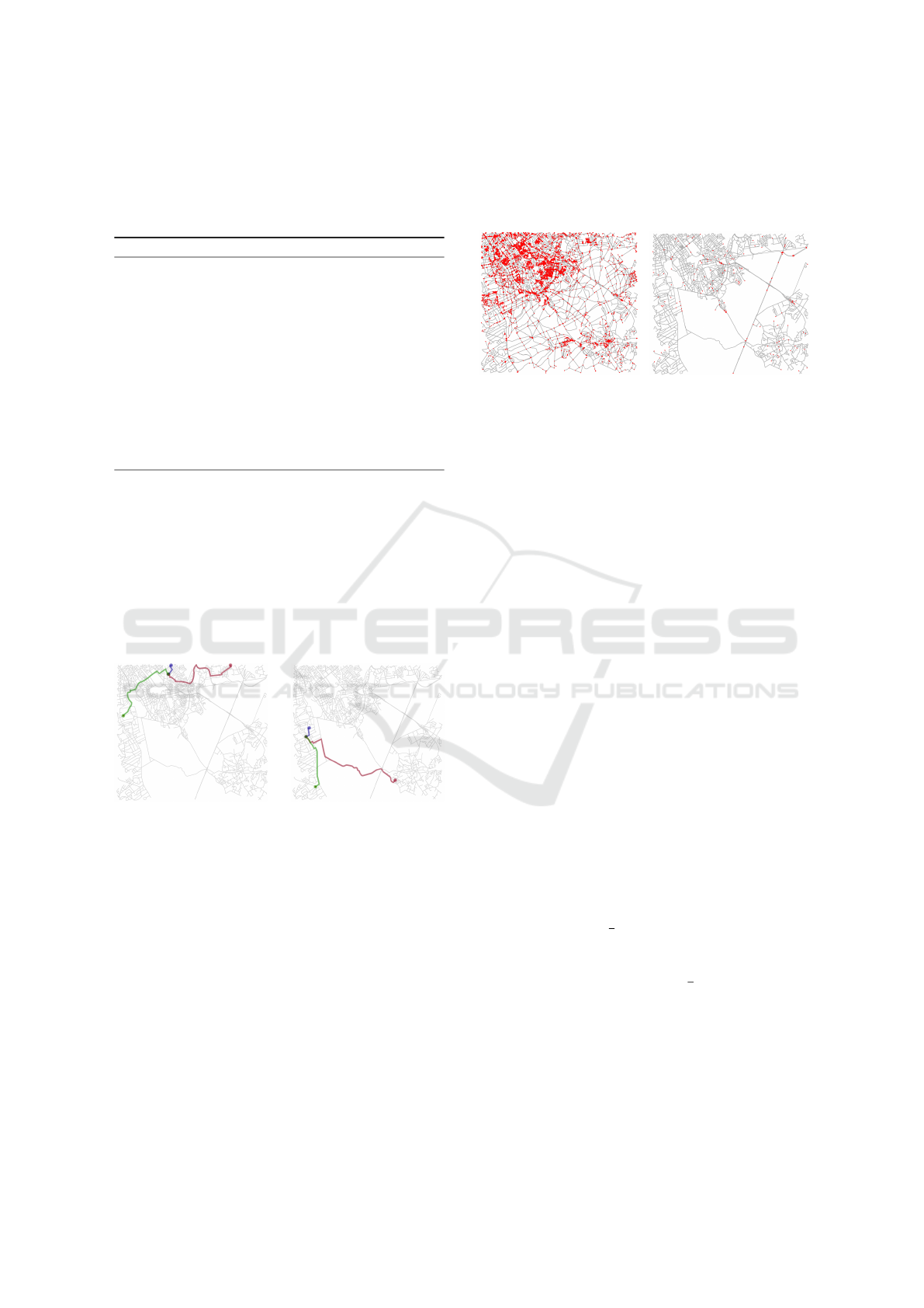
Figures 3 and 4 show practical examples of results
obtained with the algorithm 2. In red, is the path taken
by the driver u
d
, in blue is the path taken by the pedes-
trian u
w
, and in green is the path traveled together, i.e.
the actual car-sharing.
Figure 3: Example of a so-
lution N°1.
Figure 4: Example of a so-
lution N°2.
5 THE ALGORITHM
In this section, we present the proposed heuristic ver-
sion of the optimal algorithm presented in section 4
and detail the methods used to achieve faster execu-
tion.
5.1 Multimodal Pruning
To reduce the search space, we can take advantage of
the multimodal aspect of the problem. If we make
the assumption that the meeting point must be acces-
sible to both users u
w
and u
d
, we can remove all road
intersections v
i
that are not common to both users,
i.e. keeping only the nodes V = {v
1
,v
2
,..., v
n
/v
i
∈
(G
w
∩ G
d
). A simple examples of deleted nodes are
given in red in figures 5 for G
w
and in 6 for G
d
.
Figure 5: Nodes pruned to
obtain G = G
w
− (G
w
∩ G
d
)
graph.
Figure 6: Nodes pruned to
obtain G = G
d
− (G
w
∩ G
d
)
graph.
Since |G
d
− (G
w
∩ G
d
)| < |G
w
− (G
w
∩ G
d
)| there
are less nodes to delete, then the deleting process is
faster.
For the resulting graph G for the study case of
Brussels, compared with the G
w
graph, this technique
achieves an average reduction of 4.18% in the number
of nodes and 4.65% in the number of edges. How-
ever, compared with G
d
, this technique reduces the
number of nodes by 1.092% and increases the number
of edges by 1.032%. Since fewer road intersections
are accessible by car, it is preferable in terms of run-
ning time to prune the driving graph G
d
rather than
the walking graph G
w
. The major advantage of this
pruning technique is that it can be performed off-line,
but above all, the more different networks are inte-
grated, such as the network of public transport stops,
the more efficient the pruning will be, given that the
number of intersections common to all networks de-
creases with the number of transport modes taken into
account.
5.2 Heuristic Algorithm
The main idea behind the algorithm 3 is to reduce the
search space of the OMP. To achieve this, we apply
the following pre-processing: (1) First, we take the
node located at the
1
k
of the way along the shortest
path between the two users a and b on the side of the
walker, we name this intermediate node x. (2) Then,
we take the node located at the
1
k
of the way along
the shortest path between this node x and the desti-
nation d on the side of node x, and name this node
y. (3) Then, using the getNodesWithinNNeighbors
function, we retrieve all nodes that are within N steps
from the node y. (4) Finally, we give this set of nodes
to the exact algorithm 2, which searches for the OMP
in this set rather than in the entire graph. A graphi-
Heuristic Optimal Meeting Point Algorithm for Car-Sharing in Large Multimodal Road Networks
431
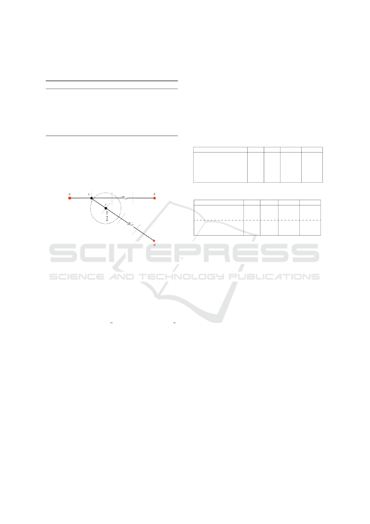
cal representation of the selection of x and y nodes is
shown in figure 7.
Algorithm 3: OMP - Heuristic algorithm.
1: SP
a,b
← di jkstra(a, b)
2: x = SP
a,b
[: len(SP
a,b
)//k]
3: SP
x,d
← di jkstra(v,d)
4: y = SP
x,d
[: len(SP
x,d
)//k]
5: neighbors ← getNodesWithinNNeighbors(N,y)
6: m ← Algorithm2(neighbors,a,b,d)
Let M = |neighbors|, V be the number of nodes in
G and a Dijkstra algorithm with a time complexity in
O
D
(V logV ). The equation 10 gives the total worst-
case complexity for the algorithm 3.
O
total
= [2 ∗ O
D
(V logV )] + [3 ∗ O
D
(M logM)] (10)
Figure 7: Node selection pre-processing for heuristic algo-
rithm.
The k value should be chosen to be closest to the
weakest or slowest user, i.e. the pedestrian. This has
the effect of reducing the search space in the zone for
which both users have an equivalent travel time. We
call this value the Xratio on the shortest path between
the two users and the Mratio for that on the shortest
path between x and the destination. In the example
of the figure 7, we have
1
k
= Xratio = Mratio =
1
4
.
Different values of k and N have been tested in sec-
tion 6.3 to assess their correctness regarding the exact
algorithm.
6 EXPERIMENTS
In this section, the various results obtained are pre-
sented. All experiments were carried out on a Win-
dows 11 machine equipped with an 8-core AMD
Rizen 7 5800X processor with a frequency of 3.80
GHz and 32 GB of RAM. For the sake of quick pro-
totyping, and despite its high resource requirements,
the various algorithms have been written in Python
3.10.11. In the current version of the code, graphs
are stored in the form of a dictionary of dictionaries
via the NetworkX library (Hagberg et al., 2008), but
this solution is far from optimal and needs to be mod-
ified in the future. For each experiment, we choose
the starting point a for the walker and b for the driver
randomly in G and we select a common destination
point d randomly in G as well.
Table 1 shows a set of small cities in Belgium.
These data were used to quickly test the results ob-
tained by the different algorithms. Table 2 shows the
properties of the different real road networks which
are also evaluated in this section.
Table 1: Benchmark of small graphs from Belgium.
G Nodes Edges Max deg Avg. deg
LOM (Lommel, Belgium) 1716 4173 8 4.86
MEC (Mechelen, Belgium) 1954 4393 8 4.50
MOU (Mouscron, Belgium) 1957 4389 8 4.49
LEV (Leuven, Belgium) 2390 5296 9 4.43
TOU (Tournai, Belgium) 2770 6407 9 4.63
MON (Mons, Belgium) 3002 6620 10 4.41
Table 2: Benchmark of large graphs.
G Nodes Edges Max deg Avg. deg
BRU (Brussels, Belgium) 3040 6961 10 4.57
BAR (Barcelona, Spain) 8870 16518 9 3.72
PAR (Paris, France) 9602 18523 10 3.86
BER (Berlin, Germany) 28003 73031 12 5.22
ROM (Rome, Italy) 43168 89595 10 4.15
NY (New York, USA) 55335 139652 11 5.05
6.1 Objective Function Evaluation
In this section, we compare the effects of the different
objective functions proposed in section 3.1.1 on the
results given by the exact solution. For each objec-
tive function, we compare the total travel time for the
passenger with the one of the driver. As in (Laupich-
ler and Sanders, 2023), we have assumed 4.5km/h for
the speed at which the passenger travels, and we take
the maximum speed allowed on the roads as the travel
speed for the driver.
Figures 8 and 9 show the difference in travel time
between the two users to reach the OMP over 100
random iterations on the different real road networks.
These figures show that for the objective functions 2
and 4, the average difference between the travel times
of the two users is smaller than in the case of the ob-
jective function 3.
Figures 10 and 11 show the difference between
the travel time of the shortest path from the source to
the destination and the travel time of the path passing
through the OMP for carpooling to join the destina-
tion. For both figures, the time differences are sepa-
rate for each user and compute over 100 random itera-
tions on the different real road networks. For three ob-
jective functions, on average, the application of a car-
sharing path is largely beneficial in terms of pedes-
trian travel time t
u
w
a,d
compared with the time it takes
VEHITS 2024 - 10th International Conference on Vehicle Technology and Intelligent Transport Systems
432
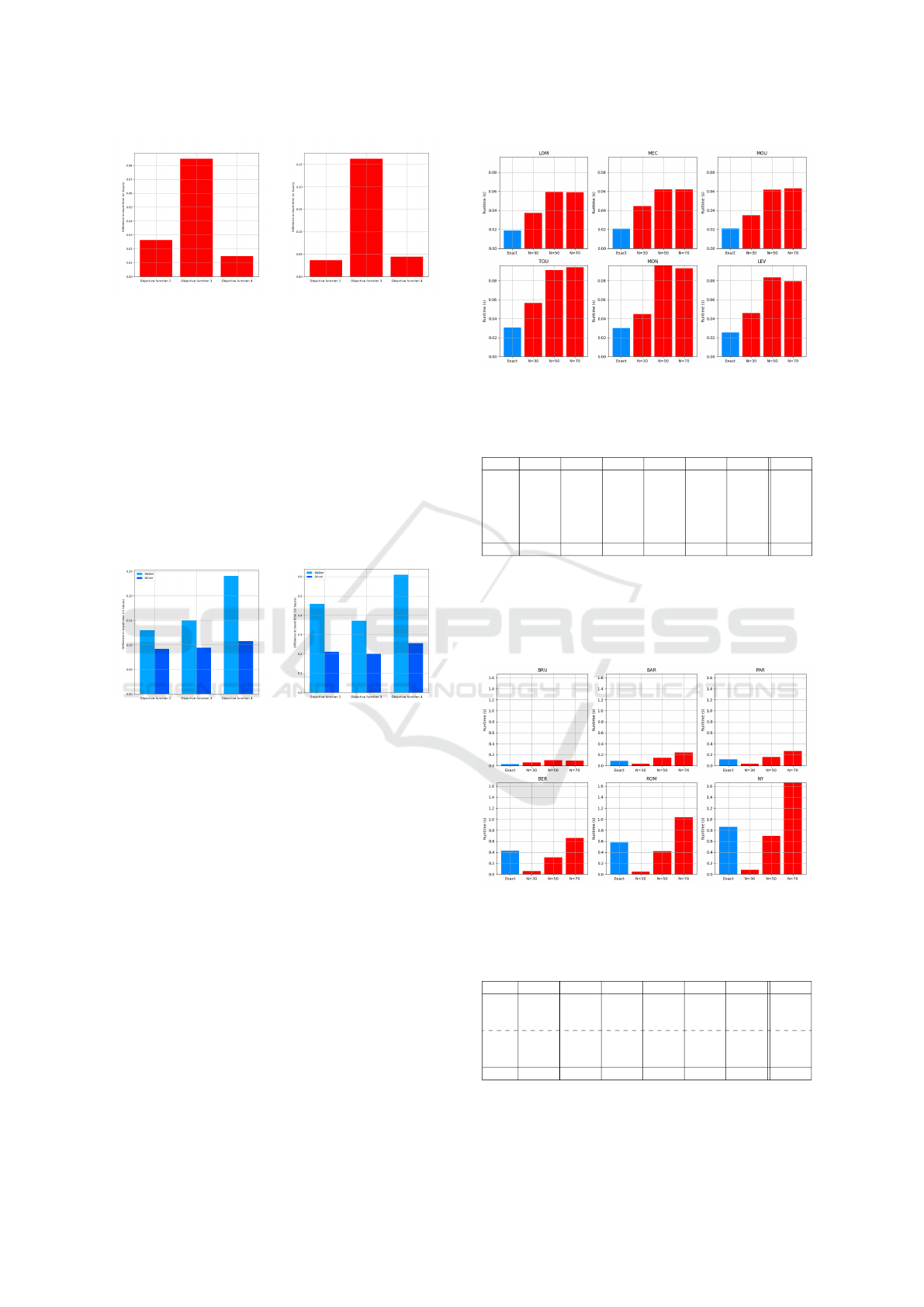
Figure 8: Difference in
travel time between driver
and walker for each the ob-
jective functions on dataset
1.
Figure 9: Difference in
travel time between driver
and walker for each the ob-
jective functions on dataset
2.
to cover the shortest route to the destination. We note
that on average car-sharing represents a loss of time
for the car user t
u
d
b,d
compared with the direct short-
est path to the destination due to a detour to OMP.
However, in practice, this difference shouldn’t be so
marked, as it is rare for cars to be able to travel at
the maximum speed allowed on the roads due to traf-
fic jams in big cities, plus regular stops at red traffic
lights and others.
Figure 10: Difference in
travel time between shortest
path and for and car-sharing
path for each the objective
functions on dataset 1.
Figure 11: Difference in
travel time between shortest
path and for and car-sharing
path for each the objective
functions on dataset 2.
In the remainder of this article, the objective func-
tion 4 has been chosen by default for the heuristic
and the exact algorithm, as it is the one that gives
the smallest difference in travel time between both
users involved in car-sharing, i.e. the fairest. Also,
this objective function allows pedestrians to save the
most time compared with their initial journey. Thus,
we extend the definition of the optimal meeting point
(OMP) to the meeting point for which the travel times
of users are fair.
6.2 Run Time
In this section, we compare the execution time of the
variants of the heuristic algorithm 3 with the exact so-
lution over 100 random iterations on the different real
road networks.
Figure 12: Average run time (seconds) on benchmark 1 for
N = 30, N = 50 and N = 70.
Table 3: Run time (seconds) on benchmark 1 depending on
N value.
G N=20 N=30 N=40 N=50 N=60 N=70 Exact
LOM 0.0214 0.0388 0.0518 0.057 0.0567 0.0587 0.0209
MEC 0.019 0.0443 0.0608 0.0601 0.0601 0.0645 0.0231
MOU 0.0161 0.0387 0.0561 0.0593 0.0626 0.0605 0.0221
LEV 0.0257 0.0533 0.0713 0.0757 0.0775 0.0755 0.0282
TOU 0.0199 0.0562 0.0818 0.0859 0.0901 0.0922 0.033
MON 0.0181 0.0537 0.0829 0.0923 0.0968 0.0987 0.0347
Total 0.02 0.0475 0.0674 0.0717 0.0739 0,075 0.027
Table 3 gives the average execution time depend-
ing on N for each graph in dataset 1. We note that on
small graphs of ≈ 2500 nodes, only the version of the
heuristic algorithm with N = 20, or less, speeds up the
time needed to find the OMP.
Figure 13: Average run time (seconds) on benchmark 2 for
N = 30, N = 50 and N = 70.
Table 4: Run time (seconds) on benchmark 2 depending on
N value.
G N=30 N=40 N=50 N=60 N=70 N=100 Exact
BRU 0.0696 0.0954 0.1006 0.1003 0.1018 0.1012 0.0356
BAR 0.06 0.1296 0.1759 0.2197 0.2717 0.2799 0.0987
PAR 0.0547 0.1181 0.1905 0.2506 0.2932 0.3028 0.1144
BER 0.1122 0.2603 0.4199 0.6353 0.7869 1.1125 0.4738
ROM 0.0948 0.2758 0.5337 0.8632 1.2001 1.5273 0.6365
NY 0.1839 0.5296 0.9135 1.3986 1.8006 2.1712 0.9224
Total 0.0958 0.2348 0.389 0.7248 0.7423 0.9158 0.3802
Table 4 gives the average execution time depend-
Heuristic Optimal Meeting Point Algorithm for Car-Sharing in Large Multimodal Road Networks
433
ing on N for each graph in dataset 2. We note that
the algorithm heuristic becomes quicker than the ex-
act algorithm for graphs with a number of nodes
|G| >≈ 10000 and values of N ≤ 50.
For both datasets, we observe that the execution
time of the heuristic algorithm depends directly on the
value of N chosen. The smaller the N, the shorter the
execution time.
6.3 Solution Correctness and Quality
In this section, we compare the results of the exact
algorithm with the results obtained by the heuristic
algorithm.
The approximation error is calculated by taking
the difference between the length of the shortest path
SP to the candidate point p for the OMP found by the
proposed algorithm and the length of the shortest path
to the exact OMP. Equation 11 formulates the error
used in the remainder of this section.
error =
|
len(SP
a,p
) − len(SP
a,omp
)
|
(11)
In other words, the error gives the difference in
number of road intersections between the solution
found by the heuristic algorithm and the solution
found by the exact algorithm. This error can therefore
reach values superior to 1.
6.3.1 Effect Xratio and Mratio on Solution
Quality
In order to evaluate which values of Xratio and
Mratio produce the best quality solutions for the
heuristic algorithm, we tested ratio values k in
[2,4, 8,12, 16,32, 64] with X ratio = Mratio over 100
random iterations on the real road networks. Fig-
ure 14 shows the average number of incorrect solu-
tions found by the heuristic algorithm with N = 50
for the dataset 1 and figure 15 shows the results for
the dataset 2 with the same values for N and k.
For dataset 1, k = 4 is the one with the smallest
errors among the test values. For dataset 2, k = 4 is
also the value for which the error is minimized. We
note that on average the number of errors is higher for
dataset 2, this is due to the value of N chosen for this
experiment, more details are given in section 6.3.2.
Thus, it seems that Xratio = Mratio =
1
4
is the opti-
mal value for the both datasets tested. Note that the
value chosen for Xratio = Mratio has no effect on the
execution time of the algorithm.
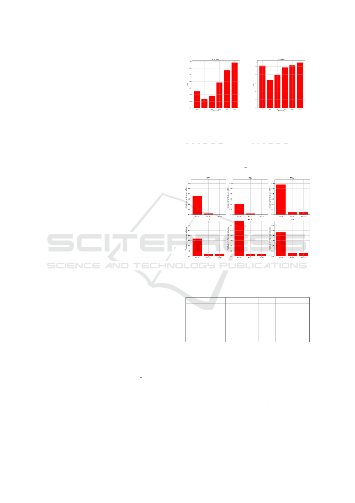
6.3.2 Effect of N on Solution Quality
Figure 16 shows the average error obtained by vari-
ants of the algorithm heuristic compared to the exact
Figure 14: Average
error of approxima-
tion on benchmark 1
for Xratio = Mratio =
[
1
2
,
1
4
,
1
8
,
1
16
,
1
32
,
1
64
].
Figure 15: Average
error of approxima-
tion on benchmark 2
for Xratio = Mratio =
[
1
2
,
1
4
,
1
8
,
1
16
,
1
32
,
1
64
].
algorithm over 100 random iterations on the dataset 1
with Xratio = Mratio =
1
4
.
Figure 16: Average error of approximation on benchmark 1
for N = 30, N = 50 and N = 70.
Table 5: Percent of correct solutions depending on N value
for 1.
Network N=20 N=30 N=40 N=50 N=60 N=70
LOM 0.52 0.82 0.95 0.99 1 1
MEC 0.51 0.9 0.99 0.99 1 1
MOU 0.39 0.71 0.9 0.98 0.98 0.98
LEV 0.46 0.77 0.91 0.97 0.97 0.97
TOU 0.38 0.83 0.97 0.98 0.98 0.98
MON 0.24 0.66 0.97 0.98 0.98 0.98
Total 0.416 0.782 0.948 0.982 0.985 0.985
Thanks to the table 5, we note that with N = 40
and over the heuristic algorithm 3 manages to find the
same solution as the exact algorithm 2 for the small
graph benchmark 1 in at least 94% of the cases, but
this is at the expense of execution time.
Figure 17 shows the average error obtained by
variants of the algorithm heuristic compared to the
exact algorithm over 100 random iterations on the
dataset 2 with Xratio = Mratio =
1
4
.
Thanks to the table 6, we note that with N = 100
and over the heuristic algorithm 3 manages to find the
same solution as the exact algorithm 2 for the large
VEHITS 2024 - 10th International Conference on Vehicle Technology and Intelligent Transport Systems
434

Figure 17: Average error of approximation on benchmark 2
for N = 30, N = 50 and N = 70.
Table 6: Percent of correct solutions depending on N value
for 2.
Network N=30 N=40 N=50 N=60 N=70 N=100
BRU 0.83 0.96 0.97 0.97 0.97 0.97
BAR 0.33 0.66 0.81 0.91 0.93 0.94
PAR 0.27 0.54 0.79 0.9 0.92 0.95
BER 0.15 0.28 0.51 0.63 0.74 0.97
ROM 0.02 0.2 0.41 0.63 0.82 1
NY 0.1 0.31 0.5 0.76 0.88 0.98
Total 0.283 0.492 0.665 0.8 0.876 0.968
graph benchmark 2 in at least 97% of the cases, but
this is at the expense of execution time.
For both datasets, the quality of the heuristic al-
gorithm solutions depends directly on the value of N
chosen, the approximation error increases as N de-
creases. Indeed, the more we extend the search area,
the more likely we are to find the OMP within it. It
can also be seen that the larger the network studied,
the higher the value of N must be chosen to achieve a
high percentage of correct solutions.
6.3.3 Trade-Off Between Solution Quality and
Runtime
The optimal value of N is the one for which the algo-
rithm is balanced between the execution time t
N
and
the error ε
N
. Thus, the optimal N satisfies the Equa-
tion 12.
N
opt
= min [Cost(N)] (12)
The cost of the heuristic algorithm is defined by
the Equation 13 where w is a weight parameter that
allows to adjust the balance between quality 1 − ε
N
and runtime.
Cost(N) = w × (1 − ε
N
) − (1 − w) ×t
N
(13)
Thanks to tables 3 and 5, we note that for smaller
networks there is no advantage in using our algorithm
instead of the exact solution as our algorithm is slower
in the majority of cases studied. However, thanks to
the tables 4 and 6 and according to the Equation 12
and 13 with w = 0.5, for large networks, we found
that N = 50 is the perfect compromise between speed
and quality among the tested value of N.
7 FUTURE WORKS AND OPEN
ACCESS
In future research, we would like to extend the scope
of this study by including more users and other modes
of transport, to better reflect real-world carpooling
conditions. It would be essential to remove the re-
quirement for users to start their journeys simultane-
ously because this constraint is not realistic in prac-
tice. It would be a good idea to take potential waiting
times for users into account. Also, it would be inter-
esting to solve this problem from the point of view of
MST or MPP and compare the results with the current
version using OMP. Finally, we would like to experi-
ment with the impact of Xratio ̸= Mratio on solution
quality, as well as more efficient data structures for
the graphs.
In order to enable repeatability of the results and
promote open science, the code is available, you can
send an email to julien.baudru@ulb.be to obtain ac-
cess to the GitHub repository.
8 CONCLUSION
We have proposed a heuristic algorithm based on the
reduction of the search space via pruning due to the
multimodal nature of carpooling and thanks to an ap-
proximation of the OMP location. We have shown
that the execution time of this heuristic algorithm does
not depend on the size of the road network on which it
is executed, unlike the exact solution. In best case for
large road networks, the proposed algorithm manages
to find the OMP 5.01 times faster than the exact so-
lution, while having an average relative error close to
1.5 in terms of road intersections. Therefore, even for
small values of N, our algorithm succeeds in finding a
solution that differs by at most 2 road intersections on
average from the exact solution. Also, we’ve shown
that our algorithm is particularly effective for road
networks with large numbers of nodes |G| >≈ 10000.
In conclusion, the proposed algorithm uses a heuris-
tic to accurately and quickly approximate the OMP by
minimizing the difference in travel times between two
users, while proposing the shortest paths for users to
join each other and then reach their common destina-
tion.
Heuristic Optimal Meeting Point Algorithm for Car-Sharing in Large Multimodal Road Networks
435

ACKNOWLEDGEMENTS
This project was supported by the FARI - AI for the
Common Good Institute (ULB-VUB), financed by the
European Union, with the support of the Brussels
Capital Region (Innoviris and Paradigm). Thanks to
Brice Petit and Lluc Bono Rossell
´
o from IRIDIA for
their feedback and suggestions.
REFERENCES
Bruglieri, M., Ciccarelli, D., Colorni, A., and Lu
`
e, A.
(2011). Poliunipool: a carpooling system for univer-
sities. Procedia - Social and Behavioral Sciences,
20:558–567. The State of the Art in the European
Quantitative Oriented Transportation and Logistics
Research – 14th Euro Working Group on Transporta-
tion & 26th Mini Euro Conference & 1st European
Scientific Conference on Air Transport.
Buchhold, V., Sanders, P., and Wagner, D. (2021). Fast,
Exact and Scalable Dynamic Ridesharing, pages 98–
112.
DIJKSTRA, E. (1959). A note on two problems in connex-
ion with graphs. Numerische Mathematik, 1:269–271.
Gedam, Celesty, Sahare, Madhavi, Sachdeo, Rajneeshkaur,
and Kulkarni, Nilima (2020). Smart transportation
based car pooling system. E3S Web Conf., 170:03004.
G
¨
arling, T., G
¨
arling, A., and Johansson, A. (2000). House-
hold choices of car-use reduction measures. Trans-
portation Research Part A: Policy and Practice,
34(5):309–320.
Hagberg, A., Swart, P., and S Chult, D. (2008). Explor-
ing network structure, dynamics, and function using
networkx. Technical report, Los Alamos National
Lab.(LANL), Los Alamos, NM (United States).
Huang, W., Zhang, Y., Shang, Z., and Yu, J. X. (2018). To
meet or not to meet: Finding the shortest paths in road
networks. IEEE Transactions on Knowledge and Data
Engineering, 30(4):772–785.
Laupichler, M. and Sanders, P. (2023). Fast many-to-
many routing for ridesharing with multiple pickup and
dropoff locations.
Li, R.-H., Qin, L., Yu, J. X., and Mao, R. (2016). Optimal
multi-meeting-point route search. IEEE Transactions
on Knowledge and Data Engineering, 28(3):770–784.
Lu
`
e, A. and Colorni, A. (2009). A software tool for com-
mute carpooling: a case study on university students
in milan. International Journal of Services Sciences -
Int J Serv Sci, 2.
Toth, P., Vigo, D., Toth, P., and Vigo, D. (2014). Vehicle
routing: Problems, methods, and applications, second
edition.
Wu, L., Xiao, X., Deng, D., Cong, G., Zhu, A. D., and
Zhou, S. (2012). Shortest path and distance queries
on road networks: An experimental evaluation. CoRR,
abs/1201.6564.
Xu, Z. and Jacobsen, H.-a. (2010). Processing proximity
relations in road networks. pages 243–254.
Yan, D., Zhao, Z., and Ng, W. (2011). Efficient algorithms
for finding optimal meeting point on road networks.
Proc. VLDB Endow., 4(11):968–979.
Yu, B., Ma, Y., Xue, M., Tang, B., Wang, B., Yan, J.,
and Wei, Y.-M. (2017). Environmental benefits from
ridesharing: A case of beijing. Applied Energy,
191:141–152.
VEHITS 2024 - 10th International Conference on Vehicle Technology and Intelligent Transport Systems
436
