Dynamic Prices in Ride-Sharing Scenarios*

Lech Duraj

and Grzegorz Herman

Theoretical Computer Science, Faculty of Mathematics and Computer Science, Jagiellonian University, Krak

ow, Poland

Keywords:

Pricing Strategy, Dynamic Pricing, Ride Sharing, Dial-a-Ride.

Abstract:

We describe a dynamic pricing strategy applicable to ride-sharing scenarios in public transportation services.

The strategy incorporates data about relation popularity and price acceptance rates. Crucially, it captures in-

terdependencies between tickets for different relations served by a single vehicle, and thus is able to balance

out locally optimal pricing with the expected future evolution of vehicle occupancy state. Based on historical

data about a real-world ride-sharing operator, we demonstrate that the proposed method is robust to imperfec-

tions in the input data, and estimate it to be more proﬁtable than both ﬁxed-price strategies (even theoretically

optimal), and an actual dynamic pricing strategy prescribed by business experts.

1 INTRODUCTION

Pricing strategies in transportation systems are an im-

portant mechanism that can be used to achieve many

different goals, like managing demand, avoiding con-

gestions, driving transportation choices, or promoting

equity. There is a vast literature on design of pricing

strategies for classical transportation systems, see for

example (Cervero, 1990; Fosgerau and Van Dender,

2013; Eliasson, 2021). Dynamic pricing strategies

were ﬁrst adopted by airline companies, and have now

become ubiquitous across various modes of trans-

portation (McGill and van Ryzin, 1999; den Boer,

2015; Selc¸uk and Avs¸ar, 2019) despite raising mul-

tiple concerns (Seele et al., 2021). Design of dynamic

pricing strategies is particularly important for intelli-

gent transportation systems (Saharan et al., 2020).

The particular case of designing pricing strategies

for bus services (Augustin et al., 2014), falls into a

more general category of pricing strategies with ﬁ-

nite horizon (Gallego and van Ryzin, 1994; DiMicco

et al., 2001; Elmaghraby and Keskinocak, 2003). The

key operational difference from other industries such

as airline services lies in offering tickets for speciﬁc

segments of the bus route rather than reserving seat

for the full route. The details of pricing strategies

used by many companies remain proprietary, with

https://orcid.org/0000-0002-0004-3751

https://orcid.org/0000-0001-6855-8316

∗

This work has been commissioned by Teroplan S.A.

and partially ﬁnanced by European Union funds (grant

number: RPMP.01.02.01-12-0572/16-01).

limited publicly available information. There are at-

tempts (Geggero et al., 2019) to analyze such strate-

gies by means of reverse engineering.

In this paper we propose a dynamic pricing al-

gorithm for long-distance ride-sharing scenarios. In

the typical scenario we have a vehicle traveling along

a prescribed route and clients booking their tickets

for a travel between chosen pickup and delivery lo-

cations in advance. The algorithm is to decide the

price offered to each individual client in an on-line

setting with uncertainty over the future demand for

the service, and over the price acceptance of the cur-

rent client. Once a client accepts the price and pays

for the ticket, the operator must guarantee a seat in the

vehicle to accommodate the travel between requested

locations. The goal of our algorithm is to maximize

the proﬁt for the operator.

In Section 2 we design a probabilistic description

that models the clients of the service. For that model

we describe an algorithm that maximizes the expected

proﬁt of the operator. In Section 3 we analyze the per-

formance of our algorithm on slightly perturbed mod-

els to show that it is not sensitive to small errors in

the model description. Finally, in Section 4 we com-

pare the proﬁts obtainable by our method with other

pricing strategies, using input data from a real-world

dial-a-ride service.

Duraj, L. and Herman, G.

Dynamic Prices in Ride-Sharing Scenarios.

DOI: 10.5220/0012722500003702

Paper published under CC license (CC BY-NC-ND 4.0)

In Proceedings of the 10th International Conference on Vehicle Technology and Intelligent Transport Systems (VEHITS 2024), pages 437-443

ISBN: 978-989-758-703-0; ISSN: 2184-495X

437

2 PRICING ALGORITHM

A data-driven dynamic pricing strategy needs to suc-

cessfully combine the following two aspects: on the

one hand, it might be computationally expensive to

compute optimal prices for each client, and on the

other, we need to be able to react to the arrival of

new clients in real time. Furthermore, the time-

dependency of the prices makes it impractical to pre-

compute them for all possible situations.

Therefore, our strategy is divided into two phases:

an ofﬂine phase in which we precompute information

in a time-independent way, and an online phase in

which we can quickly use this information to serve

the clients. The details of these phases are presented

in the following subsections.

2.1 Input Data

Before we present the details of our pricing algorithm,

let us ﬁrst discuss the data which is required to run it.

For each aspect below, we give a brief description of

how it is modeled and some intuition behind it. Pro-

viding actual high-quality model of each aspect is an

interesting research problem on its own, but these are

out of the scope of this paper. We do, however (in

Section 3), evaluate the robustness of our algorithm

with respect to the quality of the input data.

Vehicle Occupancy and Cost. Consider a vehicle

traveling along a prescribed route, picking up and

dropping off clients at various towns. It is often possi-

ble to serve a number of clients exceeding the capac-

ity of the vehicle, because some of them may travel

on non-overlapping parts of the route, and thus “share

a seat”. To capture this, we need a way of modeling

the occupancy of the vehicle.

Unfortunately, the number of possible combina-

tions of clients served by the vehicle is usually pro-

hibitively large to model explicitly. Therefore, we

propose a more general model, which may abstract

away some of the details of vehicle occupancy, while

still handling the most proﬁtable “seat sharing” situa-

tions (see also Section 5 for possible extensions).

Let the route be given as a set R of relations (i.e.,

pairs of towns). Each client, though able to specify

their exact pickup and dropoff locations, will be as-

signed to one of these relations. We model vehicle

occupancy by a ﬁnite automaton (Σ, T, η), where:

• Σ is a ﬁnite set of abstract occupancy states, with

a distinguished initial state s

corresponding to

the vehicle serving no clients (as an example, each

state might encode the number of occupied seats

on each of some coarse-grained segments of the

route),

• T is a ﬁnite set of client types, with an associ-

ated mapping τ : R → T assigning each relation

to a type (e.g., each type might correspond to a

set of route segments, with τ giving the segments

“touched” by a relation), and

• η: Σ × T → Σ is a partial transition function,

specifying how the occupancy state changes when

a client of a given type is sold a ticket (e.g., in-

crementing the number of occupied seats on each

segment of the client type).

For each state of the automaton, we also need to be

given the cost of operating the vehicle in that state.

Price Acceptance. For each relation r ∈ R and each

price, we need an estimated probability that a client

will accept the offer. It is reasonable to assume that

this probability is a non-increasing function of the

price. We require it to be given as a piecewise lin-

ear function a

: R → [0, 1] (with an arbitrary number

of pieces), called the (price) acceptance proﬁle.

Relation Popularity. Individual relations served by

the route might differ in both how they affect the vehi-

cle automaton, and in their price acceptance proﬁles.

Therefore, we need to know how popular they are,

i.e., what is the probability that a random client will

want to travel between two given locations. Please

note that we assume the relative popularity of re-

lations to be constant over time—this ﬁnite (rela-

tion) popularity distribution D : R → [0, 1], with

∑

D(r) = 1, is taken as an input.

Client Demand. We model the arrival of new

clients as a variable-rate Poisson process. The algo-

rithm is given the rate of this process, as a function ρ

of the time left until the vehicle departs from its initial

location (this is the latest moment when it is possi-

ble to offer new tickets for all relations served by the

route).

2.2 Ofﬂine Phase

The goal of the ofﬂine phase is to estimate the ex-

pected proﬁt S(s, k) from serving any given number k

of clients, starting from any given occupancy state s.

Let us take a single price acceptance proﬁle, i.e.,

a piecewise linear function a

: R → [0, 1], and con-

sider offering a price x to a client with this proﬁle.

Depending on whether they accept it or not, the ve-

hicle will transition to a new state, and thus the ex-

pected future proﬁt will change by some amount δ.

VEHITS 2024 - 10th International Conference on Vehicle Technology and Intelligent Transport Systems

438

Assume for the moment that δ is given. For an offer

x, our expected total gain including the current client

is thus a

(x) · (x + δ). In each piece, a

(x) is linear,

and therefore the gain is maximized by offering some

price ˆx

(δ), linear in δ, with the gain itself quadratic in

δ. Considering and comparing all the pieces, we form

a piecewise quadratic function g

, giving, for each δ,

the maximal expected gain from offering ˆx

(δ) for any

piece of a

We compute the function g

separately from the

price acceptance proﬁle of each relation r, and use

the relation popularity distribution D and client type

mapping τ to combine them into functions G

, one for

each client type t:

(δ) = E

(δ)| τ(r) = t ] .

Independently, we aggregate relation popularity

by client type, obtaining, for each t, the probability

that a random arriving client is of type t.

With the above information, we are now ready to

compute the pricing strategy—a two-dimensional ta-

ble, giving for each occupancy state s and each num-

ber k = 0, 1, . . . of future clients, the expected total

gain S(s, k) from optimally serving exactly k clients,

starting from state s. We compute it using dynamic

programming, as follows:

• For k = 0, no clients will arrive, so the gain is

simply the negated cost of operating the vehicle

in state s.

• For k > 0, we consider each type t of the ﬁrst

arriving client, allowed in state s. The probabil-

ity of this event is p

(these probabilities may not

sum to one, because we might not be able to serve

all types of clients). If the client accepts our of-

fer, we will transition to a new state s

′

= η(s,t),

and if not, we will remain in s. Thus, their accep-

tance would change our expected future proﬁt by

δ = S(s

′

, k − 1) − S(s, k − 1). We know that offer-

ing an optimal price (whatever it may be) in such

a case would change the proﬁt by G

(δ). Comput-

ing the expectation over all types of clients, we

obtain

S(s, k) = S(s, k − 1)+

∑

· G

(S(η(s,t), k − 1) − S(s, k − 1)).

2.3 Online Phase

Having precomputed the pricing strategy, we are

ready to serve the clients. Consider an arrival of a

client interested in traveling on relation r, happening

when the vehicle is in state s.

First, we calculate the expected number c of

clients who are yet to arrive, as the integral of the de-

mand rate function over the remaining time. Because

client arrivals are modeled as a Poisson process, from

c we can easily obtain, for each k, the probability c

that exactly k clients will yet arrive.

Should the current client accept our offer, we

would transition to a new state s

′

= η(s, τ(r)), and

expect to gain

∑

· S(s

′

, k) in the future. If they re-

ject it, we would remain in state s, and expect to gain

∑

· S(s, k) instead. Letting δ be the difference be-

tween the two values, we now offer the optimal price

from among the precomputed ˆx

(δ).

Note, that the above summation over k is formally

inﬁnite. In practice, we clip it to some ﬁnite value

K, chosen to make the tail of the Poisson distribution

negligible. K needs to be ﬁxed when the pricing strat-

egy is computed, and thus be large enough to cover

all possible values of c. Actually, one does not need

to go further than a few times the capacity of the ve-

hicle, because with a high probability of signiﬁcantly

more clients arriving, it is better to operate multiple

vehicles in parallel.

3 ROBUSTNESS

As we have already mentioned, feeding our method

with high-quality input data might be a challenging

task. It is therefore important to assess the inﬂuence

of imperfect data on the quality of the solution. To

this end, we have performed a series of simulations, in

which we have perturbed the inputs in various ways.

In each case, we have assumed the perturbed input to

model the reality, and compared the expected proﬁt

of the strategy computed using the original input with

one computed using the perturbed (“actual”) input.

3.1 Experimental Setup

Input data for all experiments was provided by Tero-

plan S.A., and comes from a real-world dial-a-ride

service Hoper operating in Poland. The route being

analyzed runs through 50 towns over a span of about

400 km, and has been split into 3 segments. The ve-

hicle considered was a 9-seater minibus with a driver,

thus able to accommodate 8 passengers. Each occu-

pancy state encoded the number of passengers carried

over each of the segments, giving a total of 9

= 729

states.

For the sake of simplicity, we have assumed that

the operating costs are independent of the passengers

served, and set them to be zero, thus optimizing the

revenue rather than the proﬁt.

Dynamic Prices in Ride-Sharing Scenarios

439

Price acceptance proﬁles for all relations served

by the route have been given the same general shape:

acceptance is constant 0.9 for prices up to some “low”

value, decreases linearly to 0.1 for prices up to some

“high” value, and ﬁnally drops linearly to 0 at some

“limit” value. The low, high, and limit values are in-

dependent for each relation, and have been speciﬁed

by business experts, based on the distance between

the endpoints of the relation, their importance, and

prices of standard (i.e., non-shared) services, if avail-

able.

Relation popularity distribution has been esti-

mated based on frequency of searches for particular

connections on the Hoper website, ﬁltered to remove

the bias caused by multiple searches for the same or

similar connection by the same user.

Relative performance of different strategies does

not depend on the absolute demand rate, but only

on the relation between its predicted and actual val-

ues. Therefore, for robustness simulations, we have

assumed the actual demand rate to be a constant func-

tion of time (e.g., one client per hour).

In each experiment, we have simulated ticket sales

for a single vehicle, over a period of 24 time units (i.e.,

24 actual clients). The rationale behind this choice

is that when the actual demand is even higher, thus

signiﬁcantly exceeding the capacity of two vehicles,

from business perspective it is better to operate two

vehicles in parallel, rather than optimize the proﬁt

from a single one. For a discussion of extending our

method to multiple vehicles, see Section 5.

3.2 Results

Details about simulation scenarios are given below—

the plots for each case present, for different values

of perturbation parameters, the relative proﬁt of the

strategy computed using original input, compared to

the one computed using the perturbed input (thus hav-

ing a perfect model of the simulated reality).

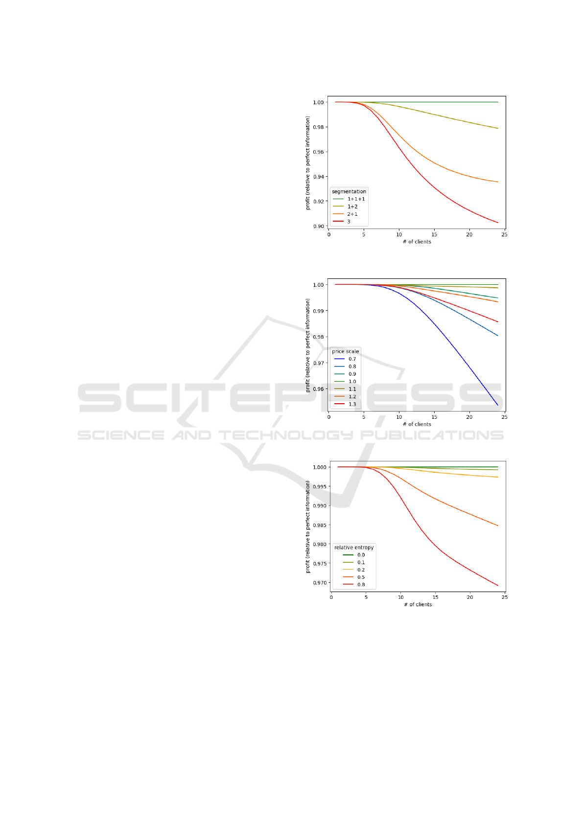
Route Segmentation. In original data, the route has

been manually divided into segments based on popu-

larity of particular destinations. We have compared

this with all possible super-segmentations, obtained

by merging some consecutive segments (or, equiva-

lently, using only a subset of the split points). The re-

sults of this experiment are shown in Figure 1 (for ex-

ample, segmentation “1+2” denotes merging the sec-

ond and third of the original segments).

Price Acceptance. In each simulation, we have

multiplied the prices in the original acceptance pro-

ﬁles by a common constant factor, thus uniformly

Figure 1: Robustness to suboptimal route segmentation.

Figure 2: Robustness to acceptable price scaling.

Figure 3: Robustness to relation popularity randomization.

scaling the prices acceptable to all clients. The in-

ﬂuence of this perturbation on the expected proﬁt is

shown in Figure 2.

Relation Popularity. To model the uncertainty in

the popularity of relations, we have assumed that the

VEHITS 2024 - 10th International Conference on Vehicle Technology and Intelligent Transport Systems

440

Figure 4: Robustness to client demand scaling.

actual popularity distribution is a random variable,

drawn from a Dirichlet distribution ∆. In each sce-

nario, we have drawn multiple samples from ∆, per-

formed independent simulations, and averaged the ex-

pected proﬁt over them. In all cases, we have assumed

the expected value of ∆ to be the original distribution

D, and varied only the concentration parameter γ.

The results of these simulations are shown in Fig-

ure 3. Because the meaning of particular values of

γ depends heavily on D, in the plots we use an al-

ternative, equivalent parameterization. For each par-

ticular γ one might calculate the expected Kullback-

Leibler divergence d

from D to a distribution ran-

domly drawn from ∆. We present d

normalized by

its maximum possible value (for our ﬁxed D)—this

way the value of zero corresponds to exactly the orig-

inal distribution, while the value of one to a mixture

of distributions, each assigning all probability mass to

a single relation (with mixture weights following the

original distribution).

Client Demand. We have perturbed the client de-

mand in two series of experiments. In the ﬁrst, we

have multiplied the demand rate by a common con-

stant factor, thus scaling it in a time-independent way.

The results of this series are presented in Figure 4.

In the second series, we have ﬁxed the total num-

ber of clients (i.e., the integral of the demand rate

function) and varied the slope of the demand rate: the

slope of 0 corresponds to the original demand rate,

the slope of −1 to there being no clients initially, but

the rate increasing linearly as the departure time ap-

proaches, and the slope of 1 to the rate being initially

maximal, but decreasing linearly to zero. The results

of this series are shown in Figure 5.

Figure 5: Robustness to client demand slope.

3.3 Discussion

As demonstrated by the experiments, our algorithm

is quite robust to imperfections in the input data. The

most important factor is the segmentation of the route,

which is not surprising, as it directly affects the num-

ber of clients we can serve at one time. However, this

is also the easiest factor to control: multiple segmen-

tations may be simulated in advance, and the best one

chosen for the actual operation—the only cost is the

size of the automaton (exponential in the number of

segments!), and consequently the time and storage re-

quired to compute the pricing strategy.

The second situation in which the algorithm per-

forms relatively poorly is when the actual demand is

signiﬁcantly lower than predicted by the model. This

suggests that any method used for demand prediction

should be calibrated to prefer underestimating the de-

mand over overestimating it.

4 PERFORMANCE

The only reliable way to compare the business per-

formance of the proposed algorithm with other meth-

ods would be a real-world A/B test. In such a test,

it is, however, not enough to split individual clients

into two groups, and offer them different prices, be-

cause the methods might attempt to balance out offer-

ing higher prices with the risk of not ﬁlling the vehi-

cle. Therefore, each vehicle would need to be fully

controlled by one of the competing algorithms. The

test would therefore require a long running time for

the results to be statistically signiﬁcant. This kind of

test is currently being prepared, but the results are not

yet available.

In the meantime, we have trained our dynamic al-

gorithm on historical data (the same used for the ro-

Dynamic Prices in Ride-Sharing Scenarios

441

bustness analysis), and performed a series of simula-

tions, in which we have compared its expected proﬁts

with each of the following:

Actual Dynamic Pricing Strategy Used by Hoper.

We used historical data provided by Teroplan S.A.,

describing actual sales of Hoper tickets for over 800

rides along the evaluated route. Tickets were dynami-

cally priced using a proprietary, expert-given strategy,

incorporating time-to-departure, current vehicle occu-

pancy, and conﬂicts between “key relations”. Unfor-

tunately, the information only contained data about

clients who have found the prices acceptable. Based

on the assumed acceptance proﬁles and relation pop-

ularity, we have used maximum likelihood estimation

for the actual client counts.

A Locally Greedy Fixed-Price Strategy. For each

relation, we use its acceptance proﬁle to determine a

price that maximizes the expected proﬁt from a sin-

gle transaction. The strategy is completely blind to

potential future clients and vehicle occupancy.

An Optimal Fixed-Price Strategy. Here, we as-

sumed perfect knowledge about the actual number of

clients. With such knowledge, for each assignment of

ﬁxed prices to individual relations, one can compute

the expected total proﬁt according to the assumed ac-

ceptance proﬁles and relation popularity. We used nu-

merical optimization to ﬁnd the best price assignment,

independently for each number of clients.

Results are compared in Figure 6. As long as the

number of clients does not exceed the capacity of the

vehicle, all evaluated strategies bring almost identical

proﬁts (the slightly lower performance of the actual

strategy used by Hoper might be a statistical ﬂuke, as

the company tried to rebook passengers from almost

empty vehicles to avoid unproﬁtable rides). Once the

demand is high enough to potentially ﬁll the vehicle,

the proﬁts of the locally optimal strategy quickly ﬂat-

ten out. Other strategies continue to bring larger prof-

its, with our proposed data-driven dynamic method

hoping to offer about a 15% gain over the one pre-

scribed by business experts.

The above performance comparison is of course

strongly dependent on the input data: the same accep-

tance proﬁles and popularity distributions are used to

compute the dynamic strategy, to evaluate the prof-

its of all three hypothetical strategies, and to esti-

mate actual client counts in historical data. The far-

ther these inputs stray from actual client behavior, the

more skewed the estimations may be. However, as we

Figure 6: Proﬁt comparison for different pricing strategies.

have demonstrated in the previous section, the pro-

posed method is quite robust to input imperfections.

In particular, save for the case of a severe overestima-

tion of the number of expected clients, the gains ex-

pected from our strategy are signiﬁcantly greater than

the expected suboptimality due to imperfect inputs.

Thus, we believe it to offer a good chance of being

proﬁtable in actual business settings.

5 CONCLUSIONS &

DIRECTIONS

We have presented here a dynamic pricing strategy

incorporating both the behavior of clients (like their

likelihood of accepting ticket prices for particular

connections) and the evolution of vehicle occupancy

in ride-sharing scenarios. While the strategy is de-

pendent on input data that might be challenging to es-

timate precisely, we have demonstrated that it is quite

robust to this input data being far from perfect—in

particular, we estimate our method to be proﬁtable

even under such imperfections.

Using a ﬁnite automaton to describe the evolution

of vehicle occupancy is very generic. In fact, it can be

used to model multiple extensions useful from busi-

ness perspective, for example:

• the cost of operating the vehicle being dependent

on the portion of the route it has to travel,

• limits on, or additional costs related to, the num-

ber of stops on the route,

• the potential proﬁtability of canceling the whole

ride (and reimbursing for tickets already sold).

We also pose the following problems for future re-

search:

VEHITS 2024 - 10th International Conference on Vehicle Technology and Intelligent Transport Systems

442

Automatic Route Segmentation. It is clear that

good segmentation of the route is crucial for the per-

formance of our algorithm. However, due to the num-

ber of possible segmentations, it is not feasible to sim-

ulate the pricing strategy for all of them. Is there a

method for ﬁnding the best segmentation (exactly or

approximately) given an upper bound on the size of

the automaton?

Furthermore, the set of occupancy states does not

need to be a Cartesian product over “atomic” seg-

ments. Knowing the popularity of particular relations,

it should be possible to merge some of the states, thus

reducing the size of the automaton or allowing to use

a ﬁner segmentation of the route.

Multiple or Larger Vehicles. Our simulations con-

sidered a single, 8-passenger vehicle. However, in

practice, it is often possible and proﬁtable to operate

multiple vehicles in parallel. Modeling two vehicles

would be approximately the same as modeling a sin-

gle 16-passenger vehicle, however this approach does

not scale well due to the growth of the automaton size.

Client Density Tuning. It is not uncommon for the

demand rate for a particular day to differ signiﬁcantly

from the average for the route due to some external

factors, which may cause our method to behave sub-

optimally. In principle, it should be possible to de-

tect such situations and adjust the expected rate dy-

namically, as the tickets are being sold—luckily, this

would not require a time-consuming recomputation of

the pricing strategy. A systematic study of this prob-

lem seems interesting.

Time-Dependent Popularity Distributions. In our

model, the relative popularity of relations is assumed

to be constant over time. However, when a route cov-

ers relations of different characteristics (e.g., long- vs.

short-distance, work- vs. leisure-related, etc.), tickets

for some of them might be systematically sought for

earlier than for others. Such an interdependence be-

tween the popularity distribution and client density

cannot be handled directly by the proposed method,

and hence requires further research.

REFERENCES

Augustin, K., Gerike, R., Martinez Sanchez, M. J., and Ay-

ala, C. (2014). Analysis of intercity bus markets on

long distances in an established and a young market:

The example of the U.S. and Germany. Research in

Transportation Economics, 48:245–254.

Cervero, R. (1990). Transit pricing research. Transporta-

tion, 17:117–139.

den Boer, A. V. (2015). Dynamic pricing and learning: His-

torical origins, current research, and new directions.

Surveys in Operations Research and Management Sci-

ence, 20(1):1–18.

DiMicco, J. M., Greenwald, A., and Maes, P. (2001). Dy-

namic pricing strategies under a ﬁnite time horizon. In

Proceedings of the 3rd ACM Conference on Electronic

Commerce, EC ’01, pages 95–104.

Eliasson, J. (2021). Efﬁcient transport pricing–why, what,

and when? Communications in Transportation Re-

search, 1:100006.

Elmaghraby, W. and Keskinocak, P. (2003). Dynamic pric-

ing in the presence of inventory considerations: Re-

search overview, current practices, and future direc-

tions. Management Science, 49:1287–1309.

Fosgerau, M. and Van Dender, K. (2013). Road pricing with

complications. Transportation, 40:479–503.

Gallego, G. and van Ryzin, G. (1994). Optimal dynamic

pricing of inventories with stochastic demand over ﬁ-

nite horizons. Management Science, 40(8):999–1020.

Geggero, A. A., Ogrzewalla, L., and Bubalo, B. (2019).

Pricing of the long-distance bus service in Europe:

The case of Flixbus. Economics of Transportation,

19:100120.

McGill, J. I. and van Ryzin, G. J. (1999). Revenue manage-

ment: Research overview and prospects. Transporta-

tion Science, 33:233–256.

Saharan, S., Bawa, S., and Kumar, N. (2020). Dynamic

pricing techniques for intelligent transportation sys-

tem in smart cities: A systematic review. Computer

Communications, 150:603–625.

Seele, P., Dierksmeier, C., Hofstetter, R., and Schultz, M. D.

(2021). Mapping the ethicality of algorithmic pricing:

A review of dynamic and personalized pricing. Jour-

nal of Business Ethics, 170:697–719.

Selc¸uk, A. M. and Avs¸ar, Z. M. (2019). Dynamic pricing in

airline revenue management. Journal of Mathematical

Analysis and Applications, 478(2):1191–1217.

Dynamic Prices in Ride-Sharing Scenarios

443