Fitting Tree Model with CNN and Geodesics to Track Blood Vessels in 2D

Medical Images and Application to Ultrasound Localization Microscopy

Data

eo Bertrand

and Laurent D. Cohen

CEREMADE, UMR CNRS 7534, University Paris Dauphine, PSL, France

Keywords:

Geodesic Methods, CNN, Vessel Tracking, ULM Imaging, Eye Fundus.

Abstract:

Segmentation of tubular structures in vascular imaging is a well studied task, although it is rare that we try

to infuse knowledge of the tree-like structure of the regions to be detected. Our work focuses on detecting

the important landmarks in the vascular network (via CNN performing both localization and classiﬁcation

of the points of interest) and representing vessels as the edges in some minimal distance tree graph. We

leverage geodesic methods relevant to the detection of vessels and their geometry, making use of the space of

positions and orientations so that 2D vessels can be accurately represented as trees. We build our model to

carry tracking on Ultrasound Localization Microscopy (ULM) data, proposing to build a good cost function

for tracking on this type of data. We also test our framework on synthetic and eye fundus data. Results show

that the Orientation Score built from ULM data yields good geodesics for tracking blood vessels but scarcity

of well annotated ULM data is an obstacle to the localization of vascular landmarks.

1 INTRODUCTION

Ultrasound Localization Microscopy is a quite recent

imaging technique that allows users to bypass the

compromise between precision and depth of penetra-

tion in ultrasound imaging.

It allows one to make highly resolved images of

the vascular network deeper in the skin tissues with

the help of micro bubbles used as contrast agents. We

refer to (Couture et al., 2018) for an overview of the

super resolution method.

In the present work, we introduce a new workﬂow

for complete end-to-end detection of vascular struc-

tures on ULM images, using deep learning to detect

landmarks (see Figure 1) allowing tracking of ves-

sels as edges in a tree graph with landmarks as ver-

tices. Our approach differs from classical Percep-

tual Grouping for blood vessel tracking as performed

in (Bekkers et al., 2018; Benmansour and Cohen,

2009). Indeed we are trying to take advantage of long

geodesics tracking blood vessels across an image, that

should behave well given the amount of literature on

the subject. While Perceptual Grouping usually fo-

cuses on computing short geodesics between close

https://orcid.org/0009-0005-7846-4985

https://orcid.org/0000-0002-3940-645X

points spread across the vessel network, we aim to

compute few long geodesics between key landmarks

of the vasculature. We try to take advandatage of the

information speciﬁcally given by ULM imaging, but

it must be noted that it is possible to adapt on other

types of images, for instance eye fundus images ob-

tained via direct photography. To do so, one may need

to evaluate local orientation information as we will

see in section 3. From a 2D image it can be done

using Orientation Scores (Duits et al., 2007) or sim-

ilar transforms such as the ones presented in (Zhang

et al., 2016) to lift a 2D image set in the plane to the 3-

dimensional space of positions and orientations. Raw

ULM data consists in ultrasound signals for imaging

blood vessels indirectly. Indeed, instead of directly

viewing the response of the tissues, it is the non-linear

response of microbubbles used as contrast agents that

is recovered and then treated to recover the position of

the bubbles. The set of the position of the microbub-

bles transported in the blood vessels allows one to

recover a highly-resolved image of the vascular tree

by projecting back on a grid as ﬁne as needed (al-

though limited by the number of detected microbub-

bles). Some methods (see for instance (Song et al.,

2018)) then use the detected points to try and recover

trajectories of microbubbles along successive images,

thus allowing one to interpolate along those trajecto-

Bertrand, T. and Cohen, L.

Fitting Tree Model with CNN and Geodesics to Track Blood Vessels in 2D Medical Images and Application to Ultrasound Localization Microscopy Data.

DOI: 10.5220/0012723900003720

Paper published under CC license (CC BY-NC-ND 4.0)

In Proceedings of the 4th International Conference on Image Processing and Vision Engineering (IMPROVE 2024), pages 44-51

ISBN: 978-989-758-693-4; ISSN: 2795-4943

ries and infer even more points in order to provide

ﬁner images. The data available and used in this work

is composed of detected trajectories of microbubbles.

We want to exploit previously recomposed trajecto-

ries by taking into account the additional information

contained in said trajectories, which are not only point

clouds but have velocity and temporal information.

Detection, segmentation or tracking tasks on med-

ical images are widely studied problems.

The contributions of our work include:

• working with ULM data, deﬁning a Riemannian

metric in order to track vessels in ULM images,

• dealing with scarcity of data : 2 different high res-

olution images to make both the training and val-

idation set,

• carrying out detection of vascular landmarks in

such context,

• ﬁtting a tree model with geodesics as edges to

take into account geometric and topological as-

pects into the tracking, thus investigating the efﬁ-

ciency of using the tree-like nature of vasculature

to perform the tracking,

• comparing results on synthetic data (hand-made

black and white images to ﬁt the framework used

for ULM data, i.e. few big images) and eye fundus

images (more images, but smaller).

Vessel segmentation is usually performed by comput-

ing scores of vesselness on the image, see the semi-

nal work (Frangi et al., 1998) and more recent work

(Jerman et al., 2016). The main idea in these works

being that high vesselness corresponds to regions in

the image where one orientation is dominant. Vessel-

ness is then deﬁned as a function of the eigenvalues

of the Hessian (in dimension 2, one eigenvalue being

signiﬁcantly higher than the other indicates a tubular

region). Modern methods of transposing the image in

a higher dimensional setting of Position-Orientation

space were used in (Zhang et al., 2016).

Other methods of vascular segmentation include

machine and deep learning methods that have become

accessible thanks to the availability of annotated data.

We can cite for instance (Oliveira et al., 2018) that

uses a fully-convolutional U-net for segmentation task

on eye fundus images.

A few works have already approached the prob-

lem of localizing vascular landmarks in eye fundus

images (Abbasi-Sureshjani et al., 2015; Pratt et al.,

2017; Wang et al., 2023; Calvo et al., 2011; Tetteh

et al., 2020) but they usually ﬁrst focus on providing

a segmentation mask of the blood vessels in the im-

age before carrying post-processing on the segmenta-

tion to infer the positions of the landmarks (endpoints,

crossings of bifurcations of blood vessels). (Hervella

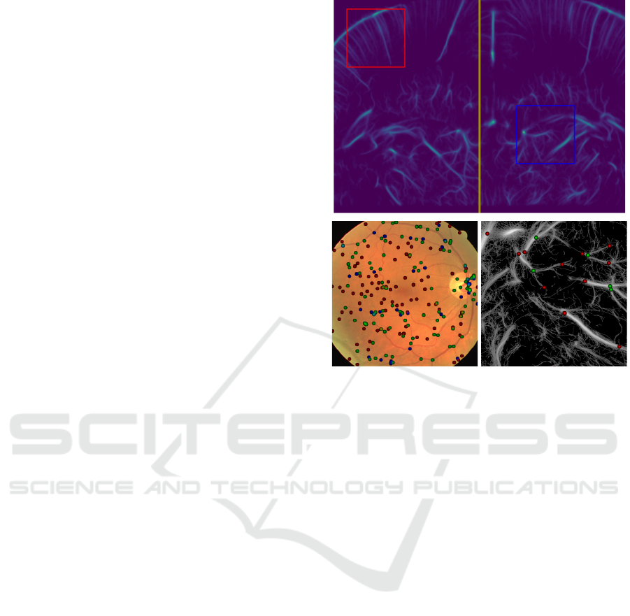
Figure 1: Top : Patches are made from a high resolution

image by cropping patches taken uniformly from each brain

half. Left : eye fundus image overlayed with heatmap of

vascular landmarks. Right : ULM image overlayed with

heatmap of vascular landmarks.

et al., 2019) tries to tackle the problem of ﬁnding

landmarks directly from input data, and we will be

building on this method here.

The second part of our workﬂow makes use

of geodesic curves to track vascular structures in

the input images. Tracking vascular structures us-

ing geodesics has been done multiple times for in-

stance in (Deschamps and Cohen, 2000; Benmansour

and Cohen, 2011), those methods have had multi-

ple extensions, for instance taking advantage of roto-

translation group (Bekkers et al., 2014) or adding ves-

sel width information (Li and Yezzi, 2007).

2 DETECTING VASCULAR

LANDMARKS

The approach to detect the vascular landmarks is very

much like the one used in (Hervella et al., 2019). The

novelty of our approach is the scarcity of ULM data

we use for learning, the integration of endpoints in

the detection task, and the tracking described further

down.

Indeed, we want to generate heatmaps with multi-

ple channels indicating probable locations of vascular

Fitting Tree Model with CNN and Geodesics to Track Blood Vessels in 2D Medical Images and Application to Ultrasound Localization

Microscopy Data

landmarks.

We train a single U-net architecture to learn the lo-

calization and classiﬁcation of interesting points in a

2D ULM image of brain vessels. The network outputs

4 channels : 3 for different types of landmarks (end-

points, bifurcations, crossings) and a last one to relax

classiﬁcation. The heatmap predicted by the CNN is

then ﬁltered to get the position of local maxima (after

thresholding at level r of output of network to reduce

noise).

2.1 ULM Data

Our data is composed of few highly resolved images

of rat brains obtained via ULM imaging. The scarcity

of data is a usual problem in medical images process-

ing. We were provided with two such images of rat

brains (two similar plans were imaged) by (Chavi-

gnon et al., 2020), we then proceeded to uniformly cut

those big (3210 × 2675) images into smaller square

patches. This way, we aggregate around 42 ULM im-

ages, making a training dataset of 21 and another set

for validation of 21 images. We make sure that there

are patches from both original images in both sets. We

also make sure that there is no overlapping between

the training and validation datasets by using different

brain halves to make those patches (see Figure 1 top).

As there is no available dataset annotation for seg-

mentation task of ULM data nor for the landmark lo-

calization and classiﬁcation task, annotation for the

latter was produced by one of the authors. The dataset

annotation was made by selecting the point landmarks

by hand with the appropriate tool (Skalski, 2019).

One great difﬁculty of our approach is that we are

highly dependent on the accuracy of the initial anno-

tation of the data which can be hard given that there

are multiple visible vessel sizes on ULM images.

To prove the efﬁcency of our method, we will

also train and evaluate our architecture on two other

datasets : one that consists in two synthetic images of

tubular structures arranged into a network, for train-

ing and validation, they are very big and are used to

imitate the case of ULM images (high resolution, few

images, thus cut into smaller patches); the other one

is simply a dataset using both images and groundtruth

from the DRIVE and IOSTAR datasets, much like in

the previously cited work (Hervella et al., 2019).

2.2 Training

The training loss is deﬁned as L(θ,x, ˆy) = ∥ f

(x) −

ˆy∥

the mean squared error (MSE), where ˆy is the

position of the labeled features in the input images

in our dataset convolved with a gaussian kernel ˆy =

∑

y∈D

∗ δ

, f

is our CNN architecture with param-

eters θ, applied on the x input image. k

is a gaussian

kernel with chosen standard deviation σ.

Going through our data we minimize the loss eval-

uated on the training set over the space of parameters

θ ∈ Θ. We may recall that the U-net architecture is

an encoder-decoder architecture composed of multi-

ple convolution layers (3 × 3 ﬁlters and leaky ReLU

activation) and with skip-connections. (Ronneberger

et al., 2015) is the fundamental work introducing this

architecture.

To make up for the small size of our dataset,

we perform data augmentation via horizontal symme-

tries, translations, rotations, all randomly applied with

predeﬁned parameters. It allows us to artiﬁcially ex-

pand our training dataset, leveraging equivariance of

our task by the action of those transformations.

3 FINDING APPROPRIATE

GEODESICS

Geodesics have been used for tracking vessels in vas-

cular images for a long time now. The works (De-

schamps and Cohen, 2000; Benmansour and Cohen,

2011) laid good basis for such work, and the book

(Peyr

e et al., 2010) that is a good introduction to the

use of geodesics for image analysis. These works

leverage our knowledge of geodesic curves and nu-

merical algorithms allowing us to compute them to

track tubular structures on medical images.

3.1 Geodesics for Vessel Tracking

Geodesics are curves that minimize a given energy

E(γ) =

P (γ(s),γ

′

(s))ds with γ ∈ Lip([0,1],Ω),

where P : Ω × R

−→ R

is some given feature po-

tential.

In fact, more than an energy, with a few hypothesis

on P , E may be seen as the length of the curve γ in

some geometry described by the potential P .

Given two points x

∈ R

, a curve minimiz-

ing the energy E under the constraints γ(0) = x

and

γ(1) = x

is called a geodesic or minimal path (joining

and x

) according to the metric deﬁned by P .

In general we will limit ourselves to the cases

where P is a Riemannian metric, i.e. the square root

of a quadratic form associated with a positive deﬁ-

nite tensor ﬁeld M : P (x,v) =

⟨

M(x)v, v

⟩

. It can

be interpreted as a local measure of the norm of some

velocity vector v in the neighbourhood of x.

The function E then deﬁnes a distance map:

IMPROVE 2024 - 4th International Conference on Image Processing and Vision Engineering

d(x,y) = inf

γ(0)=x,γ(1)=y.

E(γ). (1)

Vessel tracking can be performed by ﬁnding

geodesics on an image of the vessels. To do so, we

simply need to deﬁne a metric that is well adapted.

For now, we will restrict ourselves to Riemmanian

metrics deﬁned on the homogenous space of posi-

tions and orientations M

= R

× P

d−1

with P

d−1

≃

d−1

/{−1,1}, P

d−1

allows us to assimilate features

that have the same direction but not the same sign. we

will use the relaxed Reeds-Shepp metric that is well-

studied, Riemannian and penalizes curves that are not

planar.

The relaxed Reeds-Shepp metric is the one asso-

ciated with the metric tensor deﬁned by:

((x,θ),( ˙x,

θ))

= (2)

C((x, θ))

(| ˙x · e

| ˙x ∧ e

+ ξ

θ|

with ξ,ε ∈ R , e

the unit vector with orientation

θ. C is a cost function, in the following it will be

deﬁned as C =

1+λW

with λ = 10

and W a [0, 1]-

valued score built from the image.

This vesselness score W is important because it

allows us to associate a θ coordinate to all the de-

tected landmarks by ﬁnding the orientation θ maxi-

mizing the score at its position.

We also look to enrich our orientation-dependent

score by adding information from the detection of

vascular landmarks by imposing ∀θ,W (x,θ) = 1 if a

bifurcation has been detected at position x, so that the

landmark point is accessible from any orientation.

Similarly, if a landmark has been found and clas-

siﬁed as a crossing, we add a new point to our set of

detected points located at this position but with sec-

ond maximum intensity in the vesselness score.

Such geodesics are well-studied and have already

been used in previous works to accurately track blood

vessels (for instance in (Duits et al., 2018)). The main

asset of this model is that it helps avoid shortcuts in

the case where two different vessels cross in a 2D im-

age.

The geodesic distance can be computed efﬁciently

and fast using the Fast Marching Algorithm, we refer

to (Duits et al., 2018) and the attached library for ef-

ﬁcient computational tools used in the present work.

3.2 Clustering Landmarks Using the

Geodesic Graph

Once we have deﬁned a proper geodesic distance and

we are able to effectively compute it, we can build

a matrix D = (d(x

))

1≤i, j≤n

of pairwise distance,

where the x

are the n

detected landmarks.

This step is the computational bottleneck as it re-

quires to compute n

− 1)/2 coefﬁcients, meaning

solving n

times the Fast Marching algorithm to iter-

atively ﬁll the lines of the matrix, computing the map

d(x

,·) at every iteration i. Thus the complexity is

around O(n

N log(N)) with N the number of points.

The computed pairwise distance matrix thus de-

ﬁnes a complete weighted graph that we call the

geodesic graph. On a single image there may be

many different groups of vessels that appear, with the

computation of the pairwise distance we have already

computed the geodesic curves between each pair of

points. We then need to keep only the groups of points

that are relevant for representation of the vessels. To

cut the complete graph into smaller connected compo-

nents, we will simply perform hierarchical clustering

on the graph. Indeed, if the metric is well chosen to

make landmarks linked by the vascular network near

for the distance d, and landmarks not connected by

the vascular network far, we simply group aggregate

points that are near and separate them from the others

under some condition of threshold distance s

cluster

We may cite the work (M

ullner, 2011) as a reli-

able source for theory and algorithms for hierarchical

clustering.

3.3 Linking Landmarks Through the

Geodesic Graph

Our landmarks are now separated into multiple

groups. Each of these group supposedly represents

one connected component of the visible vascular net-

work in the 2D image.

Those smaller groups represent smaller complete

graphs, but we still need to select which of the com-

puted geodesics represent the vessels.

Now the objective is to only keep the curves that

accurately represent blood vessels in the image. This

can be done by removing some of the edges in each

smaller graph.

We need a few properties for the target graph, in-

ferred from the idea we have of the representation of

blood vessels:

• As it should represent vessels, it needs to be

”1−dimensional” i.e. it is represented by a pla-

nar graph.

• It does not have cycles.

• It is small for the geodesic distance (if previously

well chosen metric).

A good heuristic to have these properties is to look for

the minimal spanning tree in each smaller complete

graphs.

Fitting Tree Model with CNN and Geodesics to Track Blood Vessels in 2D Medical Images and Application to Ultrasound Localization

Microscopy Data

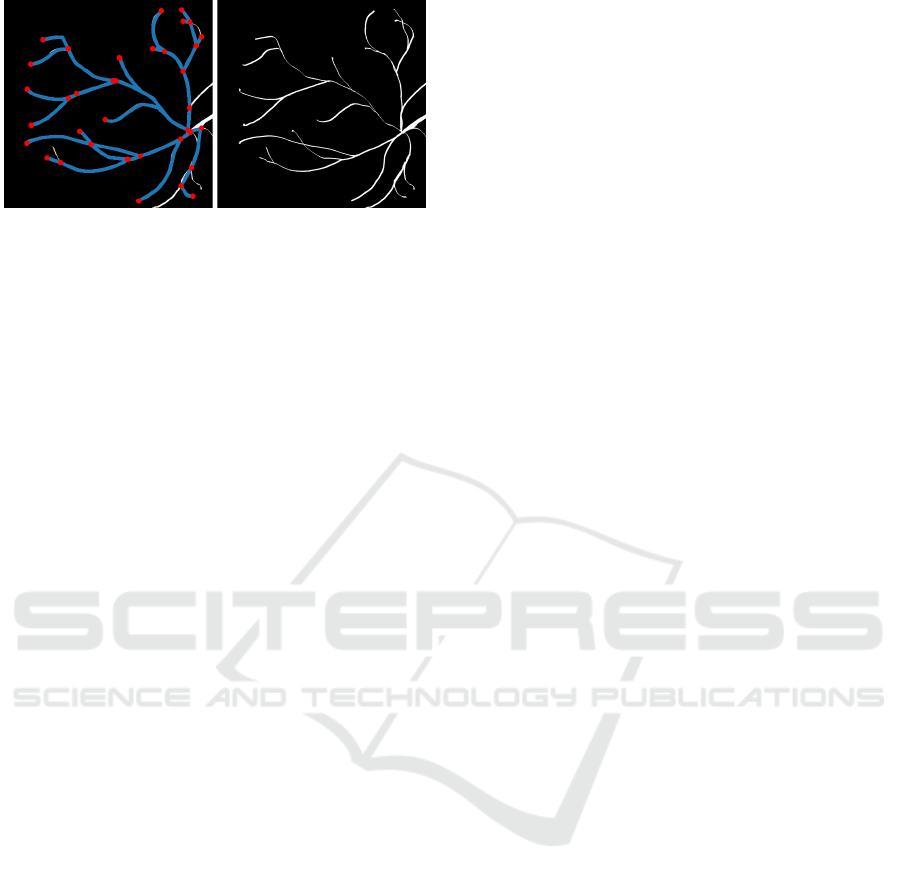
Figure 2: Geodesic graph on half of the synthetic validation

image, with N

= 128. Left image shows detected land-

marks points and the geodesics linking them, right image

shows the input image.

A few algorithms are available to perform this

computation efﬁciently. For Kruskal’s algorithm,

time complexity is of the order of the sorting of

the edges’ weights O(e log(e)) with e the number of

edges in the graph.

4 RESULTS AND DISCUSSION

4.1 Synthetic Data

To test our framework we can execute our algorithm

on synthetic hand drawn data. The main difference

is that if we use 2D images to simulate our network,

there is no straightforward way to deﬁne orientation-

lifted images as we do with ULM microbubble tra-

jectories data. To generate such orientation-lifted im-

ages, we leverage our knowledge of Orientation score

techniques.

We deﬁne a simple transformation by convolution

with the help of anisotropic gaussian kernels : the

anisotropy in a direction θ of the kernel will allow

us to select only the parts where the local features are

aligned with this direction.

This kernel deﬁnes the lifting operator Φ :

∀u ∈ L

(Ω), ∀(x,θ) ∈ Ω × [0,π[, (3)

lifted

(x,θ) = (Φu)(x,θ) = (k

lift

∗ u)(x),

To train the CNN to detect landmarks, we use two

synthetic images : one for the training set and the

other for the validation and apply the same approach

as in the case of ULM data.

Results: At the landmark-detection task level, we

were able to attain an F1 score of about 77% on the

validation dataset with hyper-parameters selected by

hand. During the training process, validation is made

on a set of images taken as random crops from the

original big image. The validation scores obtained on

those smaller (256 × 256) patches tend to give similar

scores on average along the dataset compared to eval-

uating on the whole validation image, although the

scores oscillate a lot along epochs. Figure 2 shows

the resulting tracking of synthetic vessels and the cor-

responding geodesic graph.

4.2 Eye Fundus Image

To reinforce our methodology, we apply our work-

ﬂow to a classical dataset of eye fundus images, as a

middle ground between synthetic and ULM data.

The data came from the IOSTAR and DRIVE

dataset (Abbasi-Sureshjani et al., 2015), it was split

into a training set (30 images), a validation set (10

images) and a test set (21 images).

For the training, we perform random data augmen-

tation with translations and rotations, as to avoid over-

ﬁtting and take advantage of equivariance properties

of the task at hand, and also random crops of ﬁxed

size.

We built the vesselness score W for the compu-

tation of minimal paths by ﬁrst applying a classical

Frangi ﬁlter (Frangi et al., 1998) on the input images

and then lifting the ﬁltered images via Orientation

Score as described in the previous subsection.

Results: We were able to achieve satisifying re-

sults of about 60% in F1 score on both validation

dataset and test dataset (after hyper-parameter search-

ing on the validation data). These results on the land-

marks detection task is not as good as the ones pre-

sented in (Hervella et al., 2019) but they predict only

two classes of landmarks (crossings and bifurcations)

whereas we also added the additional endpoint class.

Figure 3 shows a sample of our tracking performed on

eye fundus data.

We are able to evaluate our approach end-to-end in

the case of eye fundus data. Indeed, there is no canon-

ical way to evaluate vascular tracking versus classic

Machine Learning methods generating a segmenta-

tion mask. The most straightforward approach is to

simply project the curves on a grid of the same size

as the Ground Truth segmentation. A more sophis-

ticated approach would be to carry out the tracking

using a model taking into account the width of the

vessels during the tracking such as the ones used in

(Chen et al., 2016), but it would be necessary to lift

once again the problem to a higher dimension and the

computations would be even heavier. We use here a

simple projection method where we deﬁne a single

width and deﬁne a mask by marking all pixels at a

distance from the curves below the set width.

For the evaluation to be somewhat fair we evalu-

ate the F-score or Dice score on 24 DRIVE dataset

images and take the maximum score of the generated

IMPROVE 2024 - 4th International Conference on Image Processing and Vision Engineering

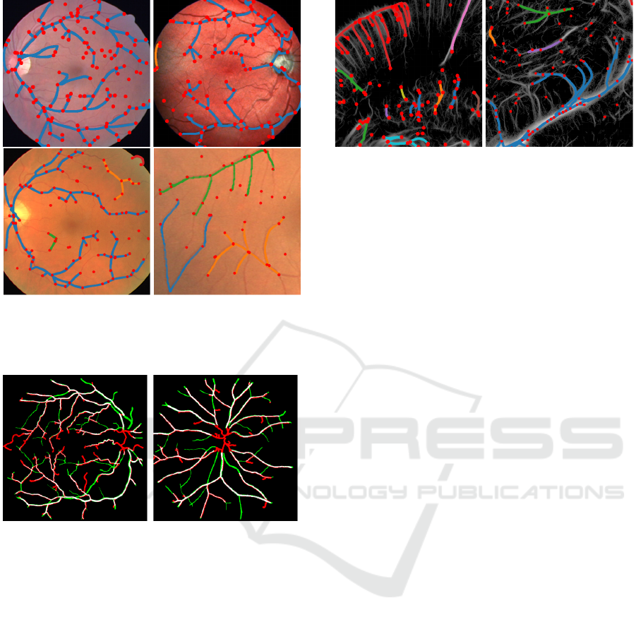
Figure 3: Geodesic tracking performed on two validation

images from the DRIVE and IOSTAR dataset, with N

64. Big red points are the detected landmarks and curves

are the selected tree structures.

Figure 4: Example of naive segmentation mask generation

from our workﬂow. Green : Ground Truth. Red : proposed

segmentation. White : the intersection.

mask with multiple widths parameters and thresh-

old in the clustering step. Thus we evaluate in fact

max

σ,s

Dice where the maximum is taken over a uni-

form grid of values for both the width and the thresh-

old in region where the optimal parameters are likely

to be located. We report an average max

σ,s

Dice score

of around 56%, which is very low compared to the ex-

pected results of much more straightforward learning

methods such as (Ronneberger et al., 2015; Liu et al.,

2022) that range between 81 and 83%.

4.3 Rat Brain ULM Data

The main ideas of the data processing for ULM data

has already been described in Section 2.

We want to make full use of ULM data and use the

initial set of microbubbles path from the available data

(Chavignon et al., 2020) to construct the cost func-

Figure 5: Geodesic graph on patches cropped from the

ULM validation dataset (taken respectively from left and

right parts of rat brain), with N

= 64. Big red points are the

detected landmarks and curves are the selected tree struc-

tures.

tion C in the relaxed Reeds-Shepp model as detailed

in Section 3.1. With this goal in mind we deﬁne W by

building directly the Orientation score from the his-

togram of microbubbles in the dataset just like it is

done for the input 2D image, but this time we add the

orientation of the given velocity vector for the orien-

tation coordinate. After renormalization it gives us a

function W (x,θ) with values beteween 0 and 1.

Results: With the described approach to learning the

detection of landmarks, we were only able to reach

low mean F1 scores of around 20 % (computed on

512 × 512 patches). Even with such a low score on

the detection-classiﬁcation task, we are able to track

a few of the vessels in the image, as shown in Figure

5. Still, some big vessels remain untracked because

some points were not found at their tips.

4.4 Discussion

Application to real world data does not seem to work

in a very satisfying way.

We may note the following behaviours observed

after training with different hyper-parameters :

• The recovery of the geodesic tree structure is

highly sensitive to change in hyper-parameters (in

the deﬁnition of the metric tensor or the depen-

dence on the position of the detected points).

• Our framework is thought for ULM images and

does not necessarily adapt well to the eye fundus

images dataset considered in the tracking step, al-

though results might get better if one can tune

the Orientation Score well enough such that ori-

entation are well separated and landmarks can be

linked i.e. reasonably close for the geodesic dis-

tance.

• Deﬁning the Orientation-dependent cost function

from the position of the microbubbles and their

estimated velocity vector seems to be a good ap-

proach to perform tracking on ULM data as we

Fitting Tree Model with CNN and Geodesics to Track Blood Vessels in 2D Medical Images and Application to Ultrasound Localization

Microscopy Data

can see from recovered geodesics in Figure 5

• The results on the synthetic images tend to show

that if we can provide a good enough segmen-

tation it would be relatively easy to provide a

good detection of landmarks and retrieve a good

geodesic tree tracking.

5 CONCLUSION AND FURTHER

WORKS

In this work we have investigated the possibility to

recover a complete tracking of the vessels in 2D im-

ages of vascular networks. It was done using CNN

techniques from the literature to extract vascular land-

marks that deﬁne the main points of interest deﬁning

the network. Our method is interesting because it ﬁts

a length-minimizing tree model to the image (using

geodesics in a certain geometry to represent vessels)

and thus includes both topological (tree-like struc-

ture) and geometrical (ﬁtting geodesics) information

to our tracking.

Although results on real world data are not satis-

fying for a complete recovery of the vasculature, nor

for segmenting the vascular network, we have shown

the potential of using ULM data and the information

they carry can be used to accurately track vessels.

Further research prospects include incorporating

scale information or scale equivariance to distinguish

vessels and help the localization process and also pro-

vide width information

ACKNOWLEDGEMENTS

This work was funded in part by the French govern-

ment under management of Agence Nationale de la

Recherche as part of the ”Investissements d’avenir”

program, reference ANR-19-P3IA-0001 (PRAIRIE

3IA Institute). The authors would to thank Dr Olivier

Couture and his team for the support on ULM data,

and Dr Erik Bekkers and Dr Jiong Zhang for the ac-

cess to the DRIVE and IOSTAR datasets.

REFERENCES

Abbasi-Sureshjani, S., Smit-Ockeloen, I., Zhang, J., and

Romeny, B. (2015). Biologically-inspired supervised

vasculature segmentation in SLO retinal fundus im-

ages. pages 325–334.

Bekkers, E., Duits, R., Berendschot, T., and ter

Haar Romeny, B. (2014). A multi-orientation anal-

ysis approach to retinal vessel tracking. Journal of

Mathematical Imaging and Vision, 49(3):583–610.

Bekkers, E. J., Chen, D., and Portegies, J. M. (2018). Nilpo-

tent Approximations of Sub-Riemannian Distances

for Fast Perceptual Grouping of Blood Vessels in 2D

and 3D. Journal of Mathematical Imaging and Vision,

60(6):882–899.

Benmansour, F. and Cohen, L. (2011). Tubular struc-

ture segmentation based on minimal path method and

anisotropic enhancement. International Journal of

Computer Vision, 92:192–210.

Benmansour, F. and Cohen, L. D. (2009). Fast Object Seg-

mentation by Growing Minimal Paths from a Single

Point on 2D or 3D Images. Journal of Mathematical

Imaging and Vision, 33(2):209–221.

Calvo, D., Ortega, M., Penedo, M. G., and Rouco, J.

(2011). Automatic detection and characterisation of

retinal vessel tree bifurcations and crossovers in eye

fundus images. Computer Methods and Programs in

Biomedicine, 103(1):28–38.

Chavignon, A., Baptiste, H., Hingot, V., Lopez, P., Eliott,

T., and Couture, O. (2020). Opulm pala.

Chen, D., Mirebeau, J.-M., and Cohen, L. D. (2016). Vessel

tree extraction using radius-lifted keypoints search-

ing scheme and anisotropic fast marching method.

Journal of Algorithms & Computational Technology,

10(4):224–234.

Couture, O., Hingot, V., Heiles, B., Muleki-Seya, P., and

Tanter, M. (2018). Ultrasound Localization Mi-

croscopy and Super-Resolution: A State of the Art.

IEEE Transactions on Ultrasonics, Ferroelectrics,

and Frequency Control, 65(8):1304–1320.

Deschamps, T. and Cohen, L. D. (2000). Minimal paths in

3D images and application to virtual endoscopy. In

Vernon, D., editor, Computer Vision — ECCV 2000,

pages 543–557, Berlin, Heidelberg. Springer Berlin

Heidelberg.

Duits, R., Felsberg, M., Granlund, G., and ter Haar Romeny,

B. (2007). Image analysis and reconstruction using a

wavelet transform constructed from a reducible rep-

resentation of the Euclidean motion group. Interna-

tional Journal of Computer Vision, 72:79–102.

Duits, R., Meesters, S. P., Mirebeau, J.-M., and Portegies,

J. M. (2018). Optimal paths for variants of the 2D and

3D reeds–shepp car with applications in image anal-

ysis. Journal of Mathematical Imaging and Vision,

60(6):816–848.

Frangi, A. F., Niessen, W. J., Vincken, K. L., and Viergever,

M. A. (1998). Multiscale vessel enhancement ﬁl-

tering. In Wells, W. M., Colchester, A., and Delp,

S., editors, Medical Image Computing and Computer-

Assisted Intervention — MICCAI’98, pages 130–137,

Berlin, Heidelberg. Springer Berlin Heidelberg.

Hervella, A., Rouco, J., Novo, J., Gonzalez, M., and Ortega,

M. (2019). Deep multi-instance heatmap regression

for the detection of retinal vessel crossings and bifur-

cations in eye fundus images. Computer Methods and

Programs in Biomedicine, 186:105201.

Jerman, T., Pernus, F., Likar, B., and Spiclin, Z. (2016). En-

hancement of Vascular Structures in 3D and 2D An-

IMPROVE 2024 - 4th International Conference on Image Processing and Vision Engineering

giographic Images. IEEE Transactions on Medical

Imaging, 35(9):2107–2118.

Li, H. and Yezzi, A. (2007). Vessels as 4-D curves: Global

minimal 4-D paths to extract 3-D tubular surfaces and

centerlines. IEEE transactions on medical imaging,

26(9):1213–1223.

Liu, W., Yang, H., Tian, T., Cao, Z., Pan, X., Xu, W., Jin,

Y., and Gao, F. (2022). Full-resolution network and

dual-threshold iteration for retinal vessel and coronary

angiograph segmentation. IEEE journal of biomedical

and health informatics, 26(9):4623–4634.

ullner, D. (2011). Modern hierarchical, agglomerative

clustering algorithms. CoRR, abs/1109.2378.

Oliveira, A., Pereira, S., and Silva, C. A. (2018). Reti-

nal vessel segmentation based on fully convolutional

neural networks. Expert Systems with Applications,

112:229–242.

Peyr

e, G., P

echaud, M., Keriven, R., and Cohen, L. D.

(2010). Geodesic Methods in Computer Vision and

Graphics. Arxiv.

Pratt, H., Williams, B., Ku, J., Vas, C., McCann, E., Al-

Bander, B., Zhao, Y., Coenen, F., and Zheng, Y.

(2017). Automatic Detection and Distinction of Reti-

nal Vessel Bifurcations and Crossings in Colour Fun-

dus Photography. Journal of Imaging, 4(1):4.

Ronneberger, O., Fischer, P., and Brox, T. (2015). U-

net: Convolutional networks for biomedical image

segmentation. In Navab, N., Hornegger, J., Wells,

W. M., and Frangi, A. F., editors, Medical Image Com-

puting and Computer-Assisted Intervention – MICCAI

2015, pages 234–241, Cham. Springer International

Publishing.

Skalski, P. (2019). Make Sense. https://github.com/

SkalskiP/make-sense/.

Song, P., Trzasko, J. D., Manduca, A., Huang, R., Kadirvel,

R., Kallmes, D. F., and Chen, S. (2018). Improved

super-resolution ultrasound microvessel imaging with

spatiotemporal nonlocal means ﬁltering and bipartite

graph-based microbubble tracking. IEEE Transac-

tions on Ultrasonics, Ferroelectrics, and Frequency

Control, 65(2):149–167.

Tetteh, G., Efremov, V., Forkert, N. D., Schneider, M.,

Kirschke, J., Weber, B., Zimmer, C., Piraud, M., and

Menze, B. H. (2020). DeepVesselNet: Vessel Seg-

mentation, Centerline Prediction, and Bifurcation De-

tection in 3-D Angiographic Volumes. Frontiers in

Neuroscience, 14:592352.

Wang, G., Huang, Y., Ma, K., Duan, Z., Luo, Z., Xiao, P.,

and Yuan, J. (2023). Automatic vessel crossing and bi-

furcation detection based on multi-attention network

vessel segmentation and directed graph search. Com-

puters in Biology and Medicine, 155:106647.

Zhang, J., Dashtbozorg, B., Bekkers, E., Pluim, J. P. W.,

Duits, R., and ter Haar Romeny, B. M. (2016). Ro-

bust retinal vessel segmentation via locally adaptive

derivative frames in orientation scores. IEEE Trans-

actions on Medical Imaging, 35(12):2631–2644.

Fitting Tree Model with CNN and Geodesics to Track Blood Vessels in 2D Medical Images and Application to Ultrasound Localization

Microscopy Data