An Information System for Training Assessment in Sports Analytics

Vanessa Meyer

, Lena Wiese

and Ahmed Al-Ghezi

Institute of Computer Science, Goethe University Frankfurt, Robert-Mayer-Str. 10, 60325 Frankfurt am Main, Germany

Keywords:

Sport Data Analytics, Human Activity Recognition, Data Visualization.

Abstract:

This paper presents an information system that analyzes and visualizes sports and human activity data. Clus-

tering is used to divide data into groups; however, the wide variation in methods for data preprocessing and

clustering makes it difﬁcult to decide on appropriate methods. Thus, for the analysis of clustering methods, we

comparatively evaluate methods for preprocessing the data in addition to the different methods for clustering.

In addition, our sports analytics information system provides an approach that is able to assign athletes to a

cluster based on their individual features and hence provides an individual training assessment compared to

the clusters obtained on the data. The proposed visualization approach in comparison to a certain cluster offers

an intuitive solution for assessing the goodness of ﬁt.

1 INTRODUCTION

Every day, a large amount of information is retrieved

and stored. To evaluate data, it has always been of

particular importance for people to compare things or

phenomena with each other based on their similarity,

to learn unknown patterns (Xu and Wunsch, 2005).

The similarity-based grouping of data plays a major

role in this kind of evaluation: the goal of clustering

methods is to ﬁnd groups of similar data objects in

data sets (Bishop and Nasrabadi, 2006). As an unsu-

pervised learning methods, unlike supervised learning

methods, there is no need for labeled target variables

in clustering. Hence, we can conveniently base our

analysis only input variables.

Advances in modern communication technologies

(through portable, mobile devices and “wearables”)

have made the areas of “individualized training mon-

itoring” and “smart health” a central part of modern

life in order to improve athletic performance and in-

dividual health. In addition to these continuously col-

lected monitoring data, there are also conventional

data collected from laboratory tests (genomics, blood

values) or questionnaires (mental health). Very com-

plex data sets are therefore available in the area of

sports and health, covering different modalities and

granularities. From an economic perspective, the

sports sector is a key growth market: “The sport-

https://orcid.org/0009-0006-3394-6291

https://orcid.org/0000-0003-3515-9209

https://orcid.org/0000-0002-1683-0629

stech industry has experienced and is expected to ex-

perience exceptional growth with a compound an-

nual growth rate of more than 20% between 2018 and

2024” (Frevel et al., 2020). The ISPO (International

Trade Fair for Sporting Goods and Sports Fashion)

even speaks of “an increase of 60 percent to around

C82.3 million” in spending on ﬁtness apps in Ger-

many in the year 2020

. The marketable goal of our

sports information system is to create personalized

recommendations for improvements in training and

health status. This is based on the analysis of clus-

ters/cohorts of similar athletes and the training rec-

ommendations that could be derived from them. As

a long-term vision such an information system may

also support commercial applications, for example for

manufacturers of ﬁtness equipment – especially in

combination with mobile devices (smart watches or

ﬁtness trackers connected to corresponding apps).

Contributions. Extending our previous work

(Meyer et al., 2023), we present an information sys-

tem to ﬁnd prototypical features in sports data using

clustering techniques while optimizing associated

methods for preprocessing the data. Our use case

is a personalized assessment of the training status

of individuals in this sports information system. To

illustrate our system, a public data set is used for test-

ing: the Multilevel Monitoring of Activity and Sleep

in Healthy people (MMASH) data set (Rossi et al.,

https://www.ispo.com/en/topic/sportstech

Meyer, V., Wiese, L. and Al-Ghezi, A.

An Information System for Training Assessment in Sports Analytics.

DOI: 10.5220/0012724200003690

Paper published under CC license (CC BY-NC-ND 4.0)

In Proceedings of the 26th International Conference on Enterprise Information Systems (ICEIS 2024) - Volume 1, pages 149-160

ISBN: 978-989-758-692-7; ISSN: 2184-4992

149

2020a; Rossi et al., 2020b) available via Physionet

(Goldberger et al., 2000). The data set is prepro-

cessed accordingly before clustering, where different

variants of method combinations are tested here.

Furthermore, the following well-known clustering

methods are used: K-Means, Hierarchical Clustering,

Density-Based Spatial Clustering of Applications

with Noise (DBSCAN), Afﬁnity propagation, Mean-

shift and Balanced Iterative Reducing and Clustering

using Hierarchies (BIRCH). By choosing different

clustering methods and preprocessing methods, the

differences between each method and the resulting

inﬂuence on the clustering results are clariﬁed.

In addition, we present the user interface of our

system where users can create their visual proﬁles

based on selected features. For the self-assessment,

their own measurement values for selected features

can be entered. Based on the entered values an as-

signment to a group is made, as well as a presentation

of the differences between the own features and the

features of other individuals belonging to the cluster.

Outline. Section 2 includes related works with dif-

ferent applications of data mining and clustering in

sports. Section 3 presents the MMASH dataset; this

is followed by a description of the steps used to pre-

process the data. In Section 4 six different cluster-

ing methods as well as three cluster validation in-

dexes are described. Furthermore, the section com-

pares and interprets the quality of the clusters formed

by the various clustering methods. Afterwards, Sec-

tion 5 presents a web user interface. Here the user

can select a dataset to create a visual proﬁle based on

selected features. In a ﬁnal conclusion, Section 6 pro-

vides an outlook for future research.

2 RELATED WORK

Related works are surveyed in the following that deal

with clustering or other methods from the ﬁeld of data

mining in sports. The related works show quite differ-

ent goals and applications of data mining techniques:

prediction of sports match results, performance im-

provement of individual athletes or teams, or determi-

nation of the market value of athletes or teams. Ac-

cording to (Cao, 2012), in the past, sports organiza-

tions relied on the experience of individuals such as

coaches or players. Over time, however, the amount

of data collected has increased, making the use of

methods such as data mining increasingly important.

In (Cao, 2012) a model is presented that focuses on

the prediction of scores of an NBA game; it is in-

tended to develop strategies in advance or can be con-

sidered for sports betting. Logistic Regression, SVM,

Artiﬁcial Neural Networks and Na

ıve Bayes are used,

and the accuracy of prediction of the mentioned mod-

els in is considered most important.

In (D’Urso et al., 2022), a fuzzy cluster model is

proposed that can be applied to different types of vari-

ables, so-called mixed data from the ﬁeld of sport.

The mixed data are, among others, quantitative, nom-

inal and time series data. Suitable dissimilarity mea-

sures are calculated for each variable, which are given

weights during the clustering process, as each vari-

able has a different relevance for the results. Through

a simulation study, it was shown that the model can

handle outliers and assign correct weights to the dis-

tance matrices. The authors apply the proposed clus-

ter model to data of football players that include both

performance and positional characteristics.

A clustering algorithm is also used in (Narizuka

and Yamazaki, 2019). The focus of this work is

on team sports, speciﬁcally football matches. The

method divides formations of the games into sev-

eral average formations, which are again divided into

speciﬁc patterns, so that the formations are clustered

across several games. The methods used in this work

are hierarchical clustering and the Delauny method. .

The data used is from J1 league football matches. Ac-

cording to the authors, the method provides a tool for

formation analysis and characterizing and thus recog-

nizing team styles in the respective sport.

K-Means clustering was used in (Shelly et al.,

2020) to divide the data collected with wearables from

athletes in the sport of American football into train-

ing groups. The formation of the training groups

was based on the individual playing requirements of

the athletes. According to the authors, the results of

the analysis were conﬁrmed when compared to tradi-

tional groupings for training in American football.

The focus in (Fister et al., 2020) is on individual

sports, such as running, cycling or triathlon, where

the time achieved is important for the quality of the

results. The authors review recent solutions regarding

post-hoc analysis. In this context, they mention per-

formance analysis, physical characteristics and ath-

letes’ behavior after a race. In their paper, the authors

achieve a robust solution based on heart rate data. It

could help athletic trainers advise their athletes to fur-

ther improve their performance and was tested on two

case studies of running athletes.

(Li et al., 2022) develop a model to assess the

physical ﬁtness of athletes, in addition to a recom-

mendation model. Results from an experiment show

a higher classiﬁcation accuracy compared to classical

methods. The authors estimate the application value,

research value and market application prospects for

ICEIS 2024 - 26th International Conference on Enterprise Information Systems

150

monitoring human ﬁtness using the presented meth-

ods to be high. In addition, the assessment method

obtained could be used to strengthen physical train-

ing in a targeted manner.

For prediction of the performance of trainings in

sports, (Li, 2022) use a generative adversarial neu-

ral network algorithm. Behavioral characteristics of

students are extracted; using a maximum pooling

method, the salient features of students are selected.

For prediction, the extracted features are subsequently

used as input to the neural network.

From an information system perspective, only few

related studies exist. From a physical education point

of view of pupils, (Feng, 2023) set up a web-based

system that applies a Decision Tree (DT) Classiﬁer

for data mining.

More generally, (Herberger and Litke, 2021) pro-

vide a literature survey with a focus on professional

football; while not describing any technical applica-

tions in detail, the authors discuss pros and cons of

sports data analytics.

For the purpose of general athlete monitoring

(Thornton et al., 2019) survey some statistical ap-

proaches with a focus on individual’s data (so-called

“within-athlete changes”) with respect to training

load. Similarly, (Sarlis et al., 2023) analyze injury-

induced impact on performance in professional bas-

ketball; whereas (de Leeuw et al., 2023) discuss the

impact of internal and external training load on re-

cuperation and devise a speciﬁc heart rate model for

professional road cycling.

As opposed to these related works, in this paper

we particularly focus on clustering as a data mining

tool and present an intuitive user interface.

3 DATA PREPROCESSING

3.1 Data Set

For test purposes we use the publicly accessible Mul-

tilevel Monitoring of Activity and Sleep in Healthy

people (MMASH) data set, which is presented in

(Rossi et al., 2020b) and can be downloaded on

the PhysioNet page (Goldberger et al., 2000). The

MMASH data set can be assigned to the ﬁeld of sports

and was published through the Open Database Li-

cense (ODbL). The authors of (Rossi et al., 2020b)

describe the MMASH data set as the ﬁrst public data

set that offers psycho-physiological features on such

a scale. Accordingly, there are already other data sets

with data such as long-term heartbeat data, but not in

connection with actigraph or psychological data. The

MMASH data set contains information over a 24-hour

period of continuous measurements, including mea-

surements of time intervals between heart beats, heart

rate measurements, and others. The data, collected by

the company BioBeats and researchers from the Uni-

versity of Pisa, includes data from a total of 22 par-

ticipants, who are adults, male and mainly students at

the University of Pisa. According to the authors of

(Rossi et al., 2020b), this represents a sample that is

as homogeneous as possible. There are 7 ﬁles for each

participant with a total of 61 features.

3.2 Preprocessing

Prior to clustering, the MMASH data set is prepro-

cessed to obtain data in a suitable form for the chosen

clustering procedures. (Kirchner et al., 2016), point

out the importance of preprocessing data before ap-

plying clustering algorithms. According to the au-

thors, ﬁnding appropriate methods for preprocessing

and their execution order is challenging. Therefore,

in this paper, three different variants of preprocessing

data are used to later show the impact of preprocess-

ing on clustering results.

Table 1: Three versions of preprocessing pipelines for

MMASH data.

Version 1 Version 2 Version 3

Missing

Values

ﬁll with

mean

ﬁll with

mean

replace

with 0

Feature

Selection

Pearson

Correla-

tion

PCA Pearson

Corre-

lation

(different

treshold)

Scaling MinMax Standard MinMax

Before the preprocessing methods can be applied

to the MMASH data set, the data are ﬁrst transformed

into a form suitable for the scikit-learn implementa-

tions

of the various clustering methods. Since time

series data are not considered in this paper, attributes

are transformed or aggregated accordingly. In addi-

tion, the original data (Rossi et al., 2020b; Rossi et al.,

2020a; Goldberger et al., 2000) are split into different

ﬁles for each participant. Finally, to put the data for

the clustering algorithms into a form where the values

of all participants are in one .csv ﬁle and in it each row

represents the attributes of an individual participant,

the ﬁles are merged into one remaining ﬁle.

The ﬁrst step of data preprocessing is ﬁnding

missing values and dealing with them. In the ﬁrst two

https://scikit-learn.org/stable/modules/clustering.html

An Information System for Training Assessment in Sports Analytics

151

versions, missing values are replaced with the corre-

sponding mean values of the attributes. In the third

version, missing values are replaced with the value

0. Outlier detection is not applied to the MMASH

data, since the data set contains very few data objects

anyway and without further domain knowledge it is

not possible to assess whether any outliers found are

really outliers. Subsequently, the dimension of the

data sets is reduced with respect to the number of at-

tributes. In the ﬁrst version, a subset of the features is

created using the Pearson correlation and a set thresh-

old, in which features with higher correlation were

removed. In the second version, Principal Compo-

nent Analysis (PCA) is used. In the third version, sub-

sets are again created using Pearson correlation, this

time setting a different threshold. To scale the data, in

the ﬁrst and third versions the MinMaxScaler, which

scales the values between 0 and 1 (0 is the minimum

of the values and 1 is the maximum of the values of an

attribute). In the second version, the StandardScaler

is used. Implementations

of scikit-learn were used

for the scaling methods.

4 CLUSTERING ANALYSIS

After the data has been preprocessed, clustering di-

vides the data into groups. Subsequently, the result-

ing clusters are visualized and evaluated using inter-

nal cluster indices. At the end, individual clusters are

described and interpreted.

4.1 Clustering Methods

• K-Means: A well-known partitioning method is

the K-means clustering method. In the K-means

method, parameter k is determined at the begin-

ning, where k is the number of groups to which

the individual data objects are to be assigned. To

determine the membership of the data objects in

the clusters, so-called centroids are determined

for each cluster and then each data object is as-

signed to the cluster whose centroid is closest

to the data object. The dispersion of the over-

all within-cluster is minimized by the iterative re-

distribution from the cluster members. In high-

dimensional spaces, however, these algorithms do

not show a good effect. This is because in high di-

mensional spaces almost all pairs of points are as

far away as the average. Thus, the distance con-

cept is poorly deﬁned in high-dimensional spaces.

https://scikit-learn.org/stable/auto examples/preproce

ssing/plot all scaling.html

Another disadvantage is that the number of clus-

ters to be formed must be speciﬁed by the user

in advance. In addition, partitioning methods are

sensitive to initialization, as well as to noise and

outliers. Partitioning methods also often get en-

tangled in local optima. Non-convex clusters of

different sizes or densities cannot be handled by

partitioning methods like k-means.

• Hierarchical Clustering: In contrast to partition-

ing algorithms such as k-means, hierarchical clus-

tering combines or splits existing clusters. This

creates a hierarchical structure that contains the

order in which the clusters are combined or di-

vided. The combination of clusters takes place in

the agglomerative approach of hierarchical clus-

tering. In this approach, the individual data ob-

jects initially belong to their own cluster, each of

which contains only the one data object. Thus,

initially there are the clusters S

, S

, ...S

with n as

the number of data objects. Subsequently, a cost

function is to ﬁnd pairs {S

, S

} that are to be com-

bined into a cluster at minimum cost. Thus S

and

are removed from the list of existing clusters

and a new cluster S

∪ S

is added. This proce-

dure is repeated until there is only one cluster that

contains all data objects. As for the cost function,

there are several variants such as complete linkage

(take maximum distance between members of two

clusters), average linkage (take average distance

between members of two clusters) and single link-

age (take minimum distance between members of

two clusters). Hierarchical procedures have the

disadvantages that once the decision to split or

merge groups has been made, no corrections can

be made, that there are poorly interpretable clus-

ter descriptors, and that the termination criterion

of this method is undeﬁned. Hierarchical meth-

ods are less effective in high dimensional spaces

due to the curse of dimensionality.

• DBSCAN: In contrast to the k-means algorithm,

which assumes a convex shape of the clusters, in

DBSCAN all shapes of clusters can occur. This

is because in DBSCAN the clusters are formed in

such a way that points from a high-density area

are in one cluster. Points that are in high den-

sity areas are also called core samples. Thus, a

cluster is a set of these core samples. For the

DBSCAN algorithm, two parameters must be set.

One parameter is the minimum number of neigh-

bor points (min samples) to call a point a core

sample. The second parameter that must be set

is eps(ilon). With eps the distance is speciﬁed in

which the neighbors of a core sample are located.

For forming clusters with a larger minimum num-

ICEIS 2024 - 26th International Conference on Enterprise Information Systems

152

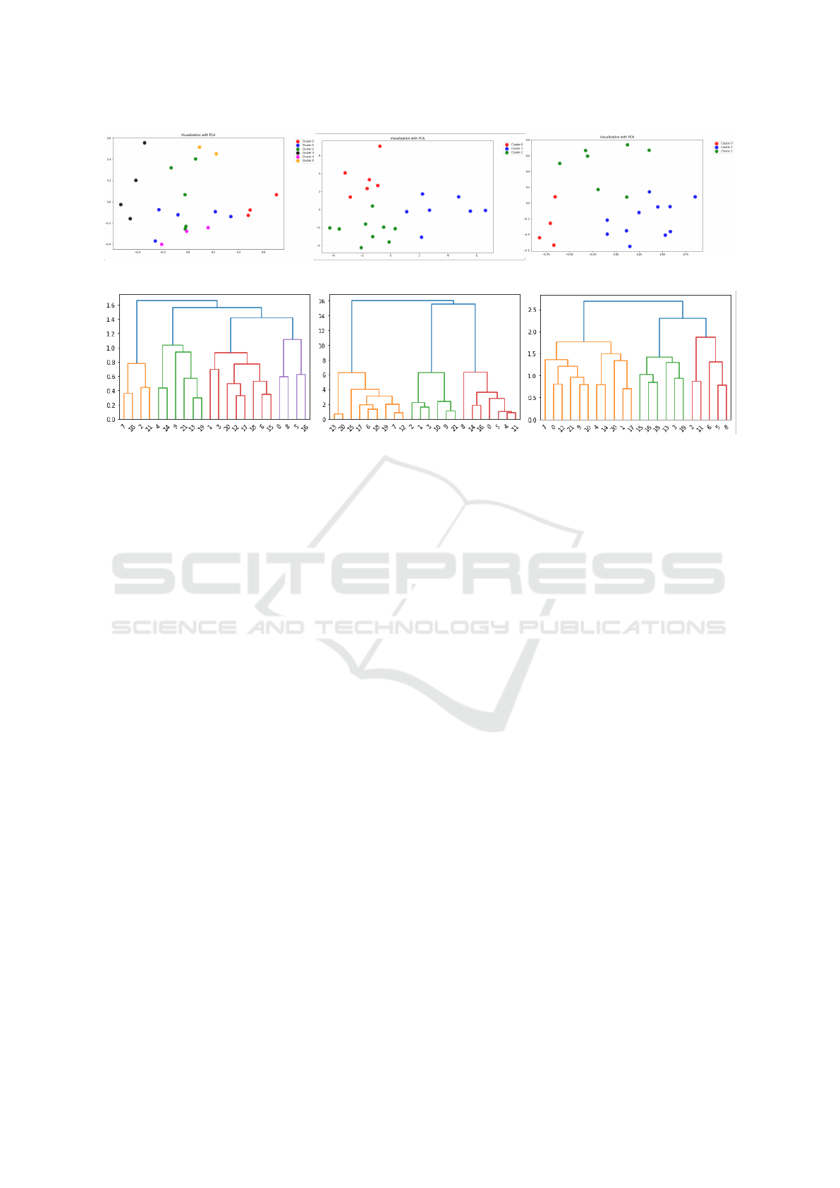
Figure 1: Resulting k-means clusters of the different data set variants (V1, V2, V3).

Figure 2: Dendrograms of the different data set variants (V1, V2, V3).

ber of neighbors or small eps, a higher density is

needed. DBSCAN starts with a random core sam-

ple and ﬁnds all its neighbors that are also core

samples. The neighboring core samples are added

to the cluster and recursively all neighboring core

samples of these newly added core samples are

added to the cluster. Neighboring non-core sam-

ples that are in the neighborhood of core samples

are also added to the cluster, but no other neigh-

bors of non-core samples are added. These Non-

core samples that are near to core samples and

thus added to a cluster are border points of the

clusters. Non-core samples that are not in the

neighborhood of core-samples are outliers. All

core-samples, however, belong to a cluster. If eps

is too small, many points are marked as outliers

with the value -1. If eps is too large, it happens

that all points are assigned to just one cluster. So,

it is important to choose an appropriate value for

the parameter eps. Advantages of density-based

cluster algorithms are that arbitrarily shaped clus-

ters can be found, the clusters found can be of dif-

ferent sizes, and their resistance to noise and out-

liers. Disadvantages are the high sensitivity to the

parameters that must be set by the user.

• Afﬁnity Propagation: In afﬁnity propagation,

messages are exchanged between pairs of sam-

ples. These exchanged messages indicate whether

a sample is suitable as an exemplar for the other

sample. Based on the responses to values of

other pairs, the suitability is iteratively updated

until convergence is reached. Once convergence

is reached, the ﬁnal clusters are formed. Based on

the given data, the number of clusters to be formed

is determined. The parameters that are important

for afﬁnity propagation are ﬁrstly the preference

and secondly the attenuation factor. The prefer-

ence controls the number of copies to be used. To

avoid numerical ﬂuctuations when updating the

responsibility and availability messages, the said

messages are damped with the damping factor.

Due to the complexity afﬁnity propagation should

rather be used for small to medium sized data sets.

• Mean-Shift: Mean-Shift is a center-based algo-

rithm that aims to ﬁnd blobs in a uniform density

of samples. In this process, candidate centers are

updated. This updating is done by having the can-

didate centers represent the mean of the points in a

region. Finally, the centers are formed by ﬁltering

the candidates in a post-processing phase to re-

move near-duplicates. The number of clusters to

be formed is determined by the algorithm. Since

the Mean-shift algorithm requires multiple near-

est neighbor searches, it is not highly scalable. In

addition, Mean-shift stops iterating at only slight

changes in centroids, but is guaranteed to con-

verge. Labeling of the new samples is done ac-

cording to the nearest centroid.

• BIRCH: In BIRCH, a feature tree is created,

where the data is compressed into cluster fea-

ture (CF) nodes containing so-called feature sub-

clusters (CF subclusters). CF subclusters, which

belong to non-terminal CF nodes, can have CF

nodes as children. The CF subclusters contain

information such as the number of samples in a

subcluster, the linear sum, squared sum, centroids,

An Information System for Training Assessment in Sports Analytics

153

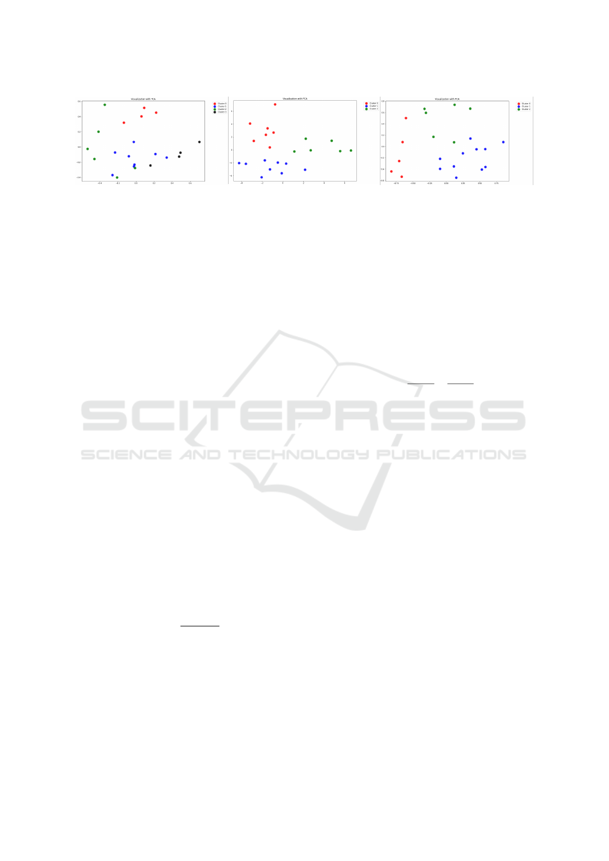
Figure 3: Resulting hierarchical clusters of the different data set variants (V1, V2, V3).

and the quadratic norm of the centroids. Thus, not

all input data need to be held in memory. The

input data is reduced to subclusters in BIRCH.

Therefore, this algorithm can also be used as an

instance or data reduction method before feeding

reduced data into a global clusterer.

4.2 Cluster Validation

After presenting some cluster algorithms, the next

step shows cluster validation indices (CVIs), which

are used and compared to measure the goodness of the

formed clusters. CVIs are used to combine compact-

ness and separability of clusters. Compactness mea-

sures the closeness of cluster elements within a clus-

ter (variance as a common measure) and separability

measures the distance between two different clusters.

In the following, some cluster validation indices are

presented based on (Rend

on et al., 2011).

• Silhouette Coefﬁcient (SC)

The Silhouette coefﬁcient is one of the evaluation

methods where the evaluation is performed us-

ing the model itself when the ground truth labels

are not present. The higher the Silhouette Score,

the better deﬁned the clusters are considered. For

each sample of the dataset, the Silhouette Coefﬁ-

cient is deﬁned by calculating the mean distance

between the sample and all other samples of the

same cluster (denoted as a in the formula below)

and the mean distance between a sample and all

other samples that are in a different, closest clus-

ter (denoted as b in the formula below). The fol-

lowing formula describes the SC s for a sample:

s =

b − a

max(a, b)

(1)

To obtain the SC for multiple samples, the aver-

age of the individual silhouette coefﬁcients of the

samples is calculated. The application of the de-

scribed SC is usually done on the results of a clus-

ter analysis. The SC can take values between -1

and 1. If the SC is around zero, this indicates over-

lapping clusters. Higher values represent denser

and more distant clusters. A disadvantage is of the

SC is that higher values are calculated for convex

clusters. Non-convex clusters, which can occur in

DBSCAN, for example, have a lower SC.

• Calinski Harabasz (CH) Index

The Calinski-Harabasz index, also called the Vari-

ance Ratio Criterion, can also be used for data sets

where there are no ground truth labels. Again, a

higher score indicates better deﬁned clusters: If

the clusters are of higher density and well sep-

arated, the CH score is higher. The Calinski-

Harabasz index is used to represent the ratio of

the sum of the dispersion between clusters and the

dispersion within clusters:

s =

tr(B

)

tr(W

)

− k

k − 1

(2)

with n

as size of data set E, k as number of clus-

ters, and traces tr of between-group dispersion

matrix B

and of within-cluster dispersion matrix

where:

∑

q=1

∑

x∈C

(x − c

)(x − c

)

(3)

with C

set of points in cluster q and c

center of

cluster q and

∑

q=1

− c

)(c

− c

)

(4)

with c

as the center of E and n

as the number

of points in cluster q. An advantage of this index

is that the values of the index can be calculated

quickly. A disadvantage is, as with the Silhouette

Coefﬁcient, that the values of the index are gener-

ally higher for convex clusters.

• Davies Bouldin (DB) Index

Analogous to the previous two validation scores,

the Davies-Bouldin index is also used when no

ground-truth labels are present. Unlike the Sil-

houette Coefﬁcient and the Calinski-Harabasz In-

dex, a lower Davies-Bouldin Index indicates that

the clusters of a model are better separated. The

average ‘similarity’ is indicated by the Davies-

Bouldin index, where this similarity is a compari-

son of the distance between clusters with the size

ICEIS 2024 - 26th International Conference on Enterprise Information Systems

154

of the clusters. The closer the values of the index

are to zero, the better the partitioning is rated, with

zero being the smallest possible and therefore best

value. Advantages of the Davies-Bouldin index

are that a simpler calculation is performed than

with the Silhouette coefﬁcient, and only pointwise

distances are used for the calculation and, conse-

quently, the index is based solely on sizes and fea-

tures inherent in the data set. A disadvantage of

this index is that the values are higher for convex

clusters than for non-convex clusters. In addition,

the distance metric is limited to Euclidean space

since the center distance is used.

DB =

∑

i=1

max

i̸= j

i j

(5)

with

i j

+ s

i j

(6)

where s

is the average distance between each

point of cluster i and the centroid of cluster i and

i j

is the distance between centroids i and j.

4.3 Clustering Comparison

Clustering was applied to the different variants of

the data set resulting from the three preprocessing

pipelines. The results are compared with respect to

the resulting clusters and cluster validation indices

Silhouette Score (SC), Calinski Harabasz Score (CH)

and the Davies Bouldin Score (DB). Based on the

results determined by the cluster validation indices,

the best possible clusters will be described and inter-

preted in more detail to perform cluster proﬁling.

• K-means: Before applying the k-means clustering

procedure to the MMASH dataset and the body

performance dataset, a suitable number of clus-

ters k is ﬁrst determined using the elbow method.

First, k-means is applied to the MMASH dataset

with preprocessing version 1. For this version,

the elbow method results in a number k = 6 of

clusters. In contrast, for the other two prepro-

cessing versions of the MMASH dataset, only

three clusters were formed. This shows that al-

ready the results of the elbow method are inﬂu-

enced by the way of preprocessing the data. In the

two-dimensional visualizations in Fig 1, which

are formed with the PCA method, it is also evi-

dent that depending on the version, the data points

are arranged differently in the coordinate system.

Hence, the components formed by PCA differ de-

pending on the version. The number of data ob-

jects in the respective cluster is shown in Table 2.

Table 2: Number of data points in the respective k-means

clusters for each data set variant.

Data Set Cl.

Cl.

MMASH V1 3 5 5 4 3 2

MMASH V2 6 7 9 - - -

MMASH V3 4 11 7 - - -

• Hierarchical Clustering: To ﬁnd a suitable num-

ber of clusters for Hierarchical Clustering, den-

drograms were ﬁrst considered. The groups high-

lighted in color in the dendrograms (Fig. 2) were

used as orientation for setting the number of clus-

ters. In this way, for the ﬁrst MMASH version,

four groups were created in the hierarchical clus-

tering. However, for the other two versions of

the MMASH dataset, three groups were created

in each case. Again, the PCA method results in

different arrangements of the data points in the

coordinate system depending on the preprocess-

ing version: Fig. 3 again shows the visualizations

of the resulting clusters of the hierarchical clus-

tering for the MMASH dataset. The number of

data objects in the respective cluster is shown in

Table 3.

Table 3: Number of data points in the respective hierarchi-

cal clusters.

Data Set Cl. 0 Cl. 1 Cl. 2 Cl. 3

MMASH V1 4 8 6 4

MMASH V2 7 9 6 -

MMASH V3 5 11 6 -

• DBSCAN: In contrast to k-means and hierarchi-

cal clustering, DBSCAN does not initially specify

a number for the groups to be formed as a parame-

ter. Here, the groups are formed during the run of

the algorithm. Given eps = 0.6 and min samples

= 2, two clusters are created for the ﬁrst version

of the MMASH dataset. For the second version

of the MMASH dataset, eps = 2 was set. The

value of min samples = 2 was also used here. This

created four clusters in the second version. The

parameters of the third preprocessing version of

the MMASH dataset were set to eps = 0.9 and

min samples = 2. Again, as in version 2, four

clusters were formed. The number of data objects

in the respective cluster is shown in Table 4.

• Afﬁnity Propagation: As with DBSCAN, no pa-

rameter for the number of clusters is set for

afﬁnity propagation. In the ﬁrst version of the

MMASH dataset, ﬁve clusters were formed by

afﬁnity propagation. In contrast, four clusters

An Information System for Training Assessment in Sports Analytics

155

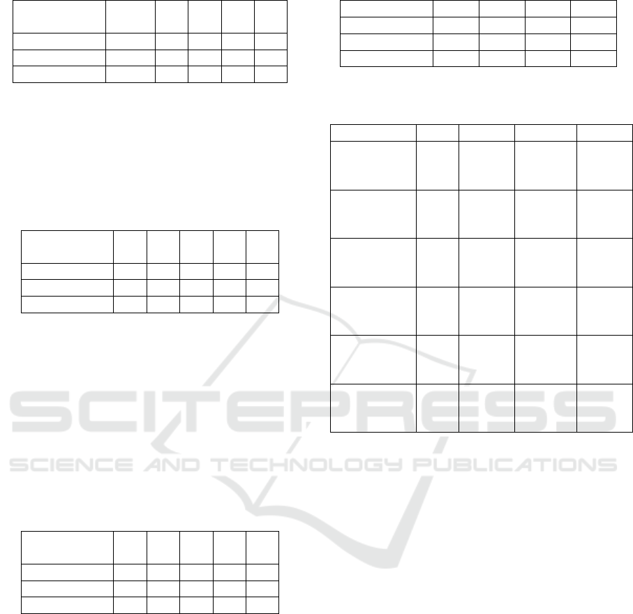
Table 4: Number of data points in the DBSCAN clusters.

Data Set Noise Cl.

Cl.

MMASH V1 3 2 17 - -

MMASH V2 2 6 3 8 3

MMASH V3 6 4 5 5 2

were formed in each of the other two versions. In

version 1 and version 3, overlaps are also evident

in some of the clusters in the visualizations. Ta-

ble 5 shows the number of data points assigned to

each cluster.

Table 5: Number of data points in the afﬁnity propagation

clusters.

Data Set Cl.

Cl.

MMASH V1 2 5 6 4 5

MMASH V2 4 7 8 3 -

MMASH V3 9 4 4 5 -

• Mean-Shift: Mean-shift also does not require the

user to specify the number of clusters. In version

1 and version 2 of the MMASH dataset, ﬁve clus-

ters were formed using mean-shift. In the third

version of the MMASH dataset, however, only

three clusters were generated using mean-shift. It

can be seen that imbalanced clusters were formed

that included very many versus very few samples.

The number of samples in the respective cluster is

shown in Table 6.

Table 6: Number of data points in the mean-shift clusters.

Data Set Cl.

Cl.

MMASH V1 15 3 2 1 1

MMASH V2 9 6 3 3 1

MMASH V3 20 1 1 - -

• BIRCH: With BIRCH, as with k-means and hier-

archical clustering, the number of clusters is cho-

sen by the user. For the MMASH dataset, four

clusters were selected as a parameter for each of

the ﬁrst two preprocessing versions. For the third

version, the parameter for the number of clusters

is set to three. Table 7 shows the respective cluster

size based on the point assignment.

The individual results of the cluster validation in-

dices (CVI) are given in Table 8 for each cluster algo-

rithm and each version of the preprocessing.

Table 7: Number of data points in the BIRCH clusters.

Data Set Cl. 0 Cl. 1 Cl. 2 Cl. 3

MMASH V1 4 8 6 4

MMASH V2 6 9 6 1

MMASH V3 5 11 6 -

Table 8: Evaluation of different cluster algorithms that were

applied to three versions of preprocessed MMASH dataset.

Algorithm CVI V1 V2 V3

K-means

SC 0.2165 0.4483 0.1568

CH 5.4768 24.6601 4.6403

DB 1.1433 0.6833 1.6557

Hierarchical

SC 0.1868 0.4674 0.1410

CH 5.3219 24.4796 4.4898

DB 1.3433 0.6445 1.6918

DBSCAN

SC 0.0768 0.3822 0.0855

CH 2.2100 10.5337 2.7669

DB 1.8793 2.2796 1.8158

Aff. Prop.

SC 0.1732 0.4185 0.0857

CH 4.5213 22.2652 3.0880

DB 1.2958 0.7266 1.7820

Mean-Shift

SC 0.0068 0.4026 0.0264

CH 2.3804 21.4384 1.5655

DB 1.1292 0.5548 0.7846

BIRCH

SC 0.1868 0.4293 0.1410

CH 5.3219 20.9996 4.4898

DB 1.3433 0.5476 1.6918

Silhouette Score: The calculated silhouette scores

for the MMASH dataset are in the positive range for

all three preprocessing combinations and all cluster

algorithms. However, the scores for all three results

are closer to the 0 value rather than the 1 value, in-

dicating that there are partially overlapping clusters.

Especially the silhouette score of version 3 is very

low and closest to 0. This could be related to the

fact that more features were retained in this version

than in the other two versions and thus the dimen-

sion of the dataset is larger and affects the goodness

of clusters. Version 2 overall has the best silhouette

scores. If only version 1 is considered and the val-

ues of the different cluster algorithms are compared,

k-means has the highest and thus best silhouette score

for version 1. In the second version, the silhouette

score for hierarchical clustering is the highest com-

pared to the other cluster algorithms. As in version 1,

k-means is also in ﬁrst place in version 3 with respect

to the silhouette score.

Calinski Harabasz Score: Overall, k-means pro-

vides the highest and thus best Calinski Harabasz

score for version 2. If only version 1 is considered,

k-means is also the algorithm that produces the high-

ICEIS 2024 - 26th International Conference on Enterprise Information Systems

156

est score for this version of the MMASH dataset com-

pared to the other cluster algorithms. For the third ver-

sion, the k-means algorithm also produces the highest

Calinski Harabasz score, although this is somewhat

lower than for version 1.

Davies Bouldin Score: For the Davies Bouldin

score, smaller values represent better separated result-

ing clusters. The closer the value is to zero, the better.

The smallest and therefore best Davies Bouldin score

for the MMASH dataset was achieved by the BIRCH

algorithm applied to version 2. For version 1 and ver-

sion 3, mean-shift produced the smallest score.

5 IMPLEMENTATION

5.1 Description of the Streamlit App

Our Streamlit web application aims to analyze data

using the K-Means clustering algorithm. Users have

the option to upload a CSV ﬁle to our application. Af-

ter uploading a CSV ﬁle, various options are available

to pre-process the data. This includes in particular

measures such as dealing with missing values and the

selection of features. It is also possible to scale se-

lected features. In addition, users can enter their own

data in additional ﬁelds in order to be assigned to a

cluster based on the entered data after the clustering

algorithm has been executed.

The libraries used in our implementation are now

explained in more detail.

Streamlit: Streamlit

is a Python library for build-

ing web applications. It is used to create our user in-

terface and interact with users.

Pandas (Python data analysis): Pandas also be-

longs to the most used libraries in the ﬁeld of Data

Science and offers among other things the possibility

to load CSV ﬁles and display them as a data frame. In

our Streamlit application it is used to read and manip-

ulate data from the CSV ﬁles uploaded by the user.

Matplotlib: Matplotlib is often used to visualize

data. We use this library to create 2D plots that visu-

alize the results of the k-means clustering algorithm.

https://docs.streamlit.io/

Scikit-learn: The scikit-learn library contains many

machine learning algorithms. Clustering and dimen-

sion reduction are among the applications of this li-

brary. In our case, it is used to perform K-Means clus-

tering and scaling data. To do this, we speciﬁcally use

sklearn.cluster.KMeans, sklearn.cluster.k means and

sklearn.preprocessing.MinMaxScaler.

NumPy (Numerical Python): NumPy is used for

numerical calculations and is considered a funda-

mental package for this. NumPy provides tools for

working with multidimensional objects (arrays) and is

widely used in data analysis. Within our application it

is used to work with arrays and numerical operations.

Plotly: The Plotly

library can be used to create in-

teractive graphs. In our streamlit application, plotly

express is used to create radar charts for cluster dis-

play with multiple features.

Seaborn: Seaborn

is based on matplotlib and is

also used to visualize data. We rely on this library

to provide a more attractive representation of data.

5.2 Data Preprocessing

After a CSV ﬁle has been successfully uploaded, the

various options for pre-processing the data become

visible. To ensure that an appropriate error message

is displayed and the user can be informed if prepro-

cessing steps are necessary before cluster analysis, the

entire preprocessing is enclosed in a try-except block.

Handling Missing Values: Using the checkbox

with the label Handling missing values, users of our

application can choose how to handle missing values

in the data set they uploaded. There are two options

to deal with the corresponding missing values. On

the one hand, missing values can be ignored, on the

other hand, missing values can be replaced by the

mean value. If the Fill with mean option is selected,

the missing values in the entire data set will be re-

placed by the mean of the respective column. Another

checkbox with the label Replace 0 with mean can be

selected if cells that contain the value 0 should also be

replaced with the mean value.

Feature Selection: In the sidebar, below the Han-

dling missing values selection ﬁelds, the features can

be selected from a list of all available features that

https://plotly.com/python/

https://seaborn.pydata.org/

An Information System for Training Assessment in Sports Analytics

157

should be used for the cluster analysis. Selected fea-

tures are stored in a separate data frame selected data.

The user can use the sidebar to choose whether the

original data or the data with the selected features

should be displayed using checkboxes. This means

that users have access to the original data and the data

with selected features at any time.

Scaling the Data: To ensure that all data have the

same scale range, the user can choose to scale the

data. If the Scale data checkbox is activated, the data

is scaled using the min-max scaling from the Scikit-

learn library. If the data has been scaled, it can also be

displayed by activating the corresponding checkbox.

Entering Individual Data: Once the user has se-

lected features that should be considered for cluster

analysis, the user can enter their own values for the

features. These values are used for assignment to one

of the resulting clusters.

5.3 Cluster Assignment

After preprocessing the data and the user’s feature in-

put, the cluster analysis can be started. To do this,

the user enters the desired number of clusters k and

starts the cluster analysis by conﬁrming the analysis

button. The K-Means algorithm from the Scikit-learn

library is run on the preprocessed data and the clus-

ter centers are determined. In addition, the values

entered by the user for the selected features are com-

pared with the descaled cluster centers (if the data was

previously scaled) so that the user can be assigned to

one of the resulting clusters. In order to compare the

data entered by the user with the calculated cluster

centers and determine a cluster assignment, the mini-

mum distance of the input vector to the cluster centers

is calculated. To do this, the np.linalg.norm method

is used, which calculates the Euclidean distance. The

following code snippet shows the cluster assignment

in more detail.

# Distances between input-vector and centers

dist = []

for center in centers_descaled:

dist.append

(np.linalg.norm(input_vector - center))

min_dist = min(dist)

assigned_Cluster = dist.index(min_dist)

The user’s entered feature values were previously

stored in an input vector array. The np.linalg.norm

function calculates the Euclidean distance between

the input vector and the descaled cluster centers (cen-

ters descaled). The array dist then contains the dis-

tances to each cluster center. Min(dist) is used to ﬁnd

the index of the minimum distance in dist. This in-

dex corresponds to the cluster that has the minimum

distance to the input vector.

5.4 Visualization Techniques

The results of the K-Means cluster analysis should be

displayed visually in order to give the user an intuitive

insight into the assignment to one of the clusters and

to clarify the differences between the individual fea-

tures and the cluster center features of the assigned

cluster. This is intended to make the interpretation

and analysis of the results easier. Radar charts and

bar charts are used for the visualization, which illus-

trate the assignment to clusters and the differences to

the cluster centers. Each selected feature is also rep-

resented by a gauge plot showing the difference be-

tween the entered values and the cluster center values.

If more than two features have been selected by

the user, a radar chart is created using the plotly li-

brary. More speciﬁcally, go.Scatterpolar (where go

stands for plotly.graph objects) is also used to display

the cluster centers and the user’s input data as lines in

the radar chart. In order to be comparable, the data is

scaled to a common scale. In the case where only two

or fewer features have been selected, a 2D bar chart

is used to visualize the results. The bar chart is also

created using the plotly library. Here go.Bar is used

to display the cluster center bars and the user’s input

data. As with the radar chart, the data from the cluster

centers and the inputs are scaled to a common scale.

After visualizing the associated cluster, the dif-

ferences of each selected feature from those of the

cluster center are shown using gauge plots using

go.Indicator. In the following section, the visualiza-

tions are shown using a sports data set as an example.

To demonstrate the visualizations, we upload the

MMASH data, which was previously converted into

a suitable format, to our Streamlit application. As an

example, ﬁve of the features were selected and the

data was scaled. After starting the analysis, we get

the following visualizations. Figure 4 shows the radar

chart, in which the features of the cluster center (of the

cluster to which the user was assigned to, based on the

entered data) and the entered user data, which were

brought to the same scale, are plotted. This means

that several features can be viewed in direct compar-

ison. However, in this type of visualization it is im-

portant that the values of all features are scaled, since

otherwise features with generally much higher values

will always be visually more pronounced in the radar

chart and the features with generally lower values will

be less pronounced in the radar chart.

ICEIS 2024 - 26th International Conference on Enterprise Information Systems

158

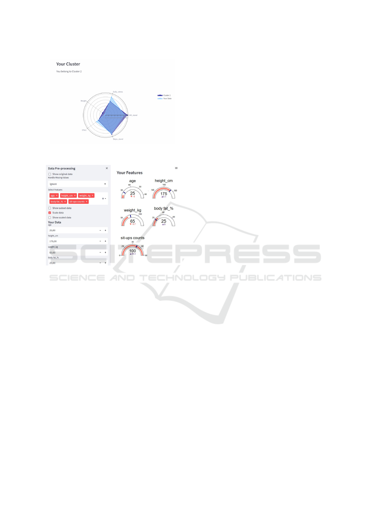
Figure 4: Visualization of a cluster and user characteristics

using a radar chart.

Figure 5: Visualization of cluster and user features using

gauge charts.

In order to be able to view the differences between

the user input and the cluster center with the actual

(unscaled) values for each feature, gauge charts as

shown in Figure 5 are used. The difference between

the user input and the value of the cluster center can

be read directly in the gauge charts. This makes it

possible to quickly assess whether a speciﬁc user fea-

ture is above or below the value of the cluster center.

6 CONCLUSIONS

Digitalization (supported by information systems) in

the ﬁelds of sports and healthcare is a strong growth

market (Schmidt, 2020) – especially through AI mod-

els, which make greater personalization and individ-

ualization possible in the ﬁrst place. Individualiza-

tion is a paradigm shift in sports analytics that is

moving towards an individualized and ﬁne-grained

evaluation of performance and health status based on

a cohort of similar athletes. The overall health of

the athletes may be analyzed through comprehensive

data analysis (laboratory tests, performance measure-

ments, blood values, but also psychological question-

naires). Individualization leads to better use of train-

ing and performance resources on the one hand and

reduces the negative side effects for athletes on the

other. In this way, our sports information system pro-

motes the innovation-driven use of data (taking mul-

timodal data types into account) by not only creating

a new business model, but also signiﬁcantly improv-

ing existing approaches (such as existing training and

health apps). The application could be further im-

proved in the future. For example, the coloring of the

visualizations (especially the radar charts) could be

optimized to make them easier to read. In addition,

other clusters (not just the cluster to which the user

was assigned) could also be used for a comparison

and displayed visually. In particular, we aim to ana-

lyze recent clustering approaches that include a deep

learning component (Karim et al., 2021) as compared

to the conventional methods used here. Furthermore,

the application could be supplemented with more de-

tailed descriptions and explanations. The preprocess-

ing options can also be further expanded in the future

by adding additional preprocessing methods.

CODE AVAILABILITY

The code of the Streamlit application is available at

https://github.com/VaneMeyer/CustomClusterVisual

izer.

ACKNOWLEDGEMENTS

This project was funded with research funds from

the Bundesinstitut f

ur Sportwissenschaften based on

a decision of Deutscher Bundestag (Project Number:

ZMI4-081901/21-25).

REFERENCES

Bishop, C. M. and Nasrabadi, N. M. (2006). Pattern recog-

nition and machine learning, volume 4. Springer.

Cao, C. (2012). Sports Data Mining Technology Used in

Basketball Outcome Prediction. Master’s thesis, Tech-

nological University Dublin.

de Leeuw, A.-W., Heijboer, M., Verdonck, T., Knobbe, A.,

and Latr

e, S. (2023). Exploiting sensor data in pro-

fessional road cycling: personalized data-driven ap-

proach for frequent ﬁtness monitoring. Data Mining

and Knowledge Discovery, 37(3):1125–1153.

D’Urso, P., De Giovanni, L., and Vitale, V. (2022). A robust

method for clustering football players with mixed at-

tributes. Annals of Operations Research, pages 1–28.

An Information System for Training Assessment in Sports Analytics

159

Feng, J. (2023). Designing an artiﬁcial intelligence-based

sport management system using big data. Soft Com-

puting, 27(21):16331–16352.

Fister, I., Fister, D., Deb, S., Mlakar, U., Brest, J., and Fis-

ter Jr., I. (2020). Post hoc analysis of sport perfor-

mance with differential evolution. Neural Computing

and Applications, 32(15):10799–10808.

Frevel, N., Schmidt, S. L., Beiderbeck, D., Penkert, B.,

and Subirana, B. (2020). Taxonomy of sportstech.

21st Century Sports: How Technologies Will Change

Sports in the Digital Age, pages 15–37.

Goldberger, A. L., Amaral, L. A., Glass, L., Hausdorff,

J. M., Ivanov, P. C., Mark, R. G., Mietus, J. E., Moody,

G. B., Peng, C.-K., and Stanley, H. E. (2000). Phys-

iobank, physiotoolkit, and physionet: components of

a new research resource for complex physiologic sig-

nals. circulation, 101(23):e215–e220.

Herberger, T. A. and Litke, C. (2021). The impact of big

data and sports analytics on professional football: A

systematic literature review. Digitalization, digital

transformation and sustainability in the global econ-

omy: risks and opportunities, pages 147–171.

Karim, M. R., Beyan, O., Zappa, A., Costa, I. G., Rebholz-

Schuhmann, D., Cochez, M., and Decker, S. (2021).

Deep learning-based clustering approaches for bioin-

formatics. Brieﬁngs in bioinformatics, 22(1):393–

415.

Kirchner, K., Zec, J., and Deliba

c, B. (2016). Facili-

tating data preprocessing by a generic framework: a

proposal for clustering. Artiﬁcial Intelligence Review,

45(3):271–297.

Li, G. (2022). Construction of Sports Training Performance

Prediction Model Based on a Generative Adversarial

Deep Neural Network Algorithm. Computational In-

telligence and Neuroscience, 2022.

Li, X., Chen, X., Guo, L., and Rochester, C. A. (2022). Ap-

plication of Big Data Analysis Techniques in Sports

Training and Physical Fitness Analysis. Hindawi

Wireless Communications and Mobile Computing Vol-

ume 2022, Article ID 3741087.

Meyer, V., Al-Ghezi, A., and Wiese, L. (2023). Exploiting

clustering for sports data analysis: A study of public

and real-world datasets. In International Workshop on

Machine Learning and Data Mining for Sports Ana-

lytics, pages 191–201. Springer.

Narizuka, T. and Yamazaki, Y. (2019). Clustering algorithm

for formations in football games. Scientiﬁc Reports,

9(1):1–8.

Rend

on, E., Abundez, I. M., Gutierrez, C., Zagal, S. D.,

Arizmendi, A., Quiroz, E. M., and Arzate, H. E.

(2011). A comparison of internal and external cluster

validation indexes. In Proceedings of the 2011 Ameri-

can Conference, San Francisco, CA, USA, volume 29,

pages 1–10.

Rossi, A., Da Pozzo, E., Menicagli, D., Tremolanti, C.,

Priami, C., Sirbu, A., Clifton, D., Martini, C., and

Morelli, D. (2020a). Multilevel monitoring of activ-

ity and sleep in healthy people. PhysioNet.

Rossi, A., Da Pozzo, E., Menicagli, D., Tremolanti, C.,

Priami, C., S

ırbu, A., Clifton, D. A., Martini, C.,

and Morelli, D. (2020b). A public dataset of 24-h

multi-levels psycho-physiological responses in young

healthy adults. Data, 5(4):91.

Sarlis, V., Papageorgiou, G., and Tjortjis, C. (2023). Sports

analytics and text mining nba data to assess recovery

from injuries and their economic impact. Computers,

12(12):261.

Schmidt, S. L. (2020). 21st Century Sports. Springer.

Shelly, Z., Burch, R. F., Tian, W., Strawderman, L., Piroli,

A., and Bichey, C. (2020). Using K-means Clustering

to Create Training Groups for Elite American Foot-

ball Student-athletes Based on Game Demands. Inter-

national Journal of Kinesiology and Sports Science,

8(2):47–63.

Thornton, H. R., Delaney, J. A., Duthie, G. M., and Das-

combe, B. J. (2019). Developing athlete monitoring

systems in team sports: Data analysis and visualiza-

tion. International journal of sports physiology and

performance, 14(6):698–705.

Xu, R. and Wunsch, D. (2005). Survey of Clustering Al-

gorithms. IEEE Transactions on Neural Networks,

16(3):645–678.

ICEIS 2024 - 26th International Conference on Enterprise Information Systems

160