A Comparative Analysis of EfﬁcientNet Architectures for Identifying

Anomalies in Endoscopic Images

Alexandre C. P. Pessoa

1 a

, Darlan B. P. Quintanilha

1 b

, Jo

ao Dallyson Sousa de Almeida

1 c

Geraldo Braz Junior

1 d

, Anselmo C. de Paiva

1 e

and Ant

onio Cunha

2 f

ucleo de Computac

ao Aplicada, Universidade Federal do Maranh

ao (UFMA), S

ao Lu

ıs, MA, Brazil

Universidade de Tr

as-os-Montes e Alto Douro (UTAD), Vila Real, Portugal

Keywords:

Endoscopy, Wireless Capsule Endoscopy, Deep Learning, EfﬁcientNet.

Abstract:

The gastrointestinal tract is part of the digestive system, fundamental to digestion. Digestive problems can be

symptoms of chronic illnesses like cancer and should be treated seriously. Endoscopic exams in the tract make

detecting these diseases in their initial stages possible, enabling an effective treatment. Modern endoscopy

has evolved into the Wireless Capsule Endoscopy procedure, where patients ingest a capsule with a camera.

This type of exam usually exports videos up to 8 hours in length. Support systems for specialists to detect and

diagnose pathologies in this type of exam are desired. This work uses a rarely used dataset, the ERS dataset,

containing 121.399 labelled images, to evaluate three models from the EfﬁcientNet family of architectures

for the binary classiﬁcation of Endoscopic images. The models were evaluated in a 5-fold cross-validation

process. In the experiments, the best results were achieved by EfﬁcientNetB0, achieving average accuracy and

F1-Score of, respectively, 77.29% and 84.67%.

1 INTRODUCTION

The gastrointestinal (GI) tract is part of the diges-

tive system, being fundamental in digestion, break-

ing down food, and absorbing nutrients. Digestive is-

sues such as bloating, constipation, or even diarrhoea

can be symptoms of chronic diseases such as cancer

and should be treated seriously. Cancers related to

the GI tract (esophageal, gastric, and colorectal, for

example) are some of the most common worldwide,

corresponding to 9.6% of cancer cases in the world,

with the second highest mortality rate (IARC/WHO,

2022b).

Worldwide, this type of cancer has the third high-

est incidence rate but has the second highest mortality

rate among cancer types, being more than 8%, with

lung cancer being the only one with a higher mortal-

ity rate. In Brazil speciﬁcally, 27% of the population

is afﬂicted with some disease in the gastrointestinal

https://orcid.org/0000-0003-4995-8909

https://orcid.org/0000-0001-8134-4873

https://orcid.org/0000-0001-7013-9700

https://orcid.org/0000-0003-3731-6431

https://orcid.org/0000-0003-4921-0626

https://orcid.org/0000-0002-3458-7693

tract. Colorectal cancer is among the three most com-

mon types of cancer among the entire Brazilian popu-

lation, surpassing the number of cases of lung cancer

(IARC/WHO, 2022a). The absence of speciﬁc symp-

toms in the initial stages results in delays in the diag-

nosis and treatment, with the prognosis of this disease

being strongly associated with the stage at which it

was diagnosed (Yeung et al., 2021).

By examining the interior of the GI tract, cancer

can be detected at an early stage, allowing for an ef-

fective treatment. The patient survival rate reaches

90% if it is diagnosed at an early stage. However, this

proportion drops to 14% in the case of an advanced-

stage cancer diagnosis (Siegel et al., 2020). Thus, en-

doscopy is one of the most used techniques for detect-

ing and analyzing anomalies in the GI tract.

However, traditional endoscopies are character-

ized by being invasive and somewhat painful, and

some complications, although rare, can include ex-

cessive sedation, perforations, hemorrhages, and in-

fections in general (Kavic and Basson, 2001). Con-

sequently, modern endoscopy has evolved into the

Wireless Capsule Endoscopy (WCE) procedure over

the past two decades. This exam consists of a pa-

tient ingesting a capsule a few millimetres in diame-

ter, coupled with a camera, a light source, a wireless

530

Pessoa, A., Quintanilha, D., Sousa de Almeida, J., Braz Junior, G., C. de Paiva, A. and Cunha, A.

A Comparative Analysis of EfﬁcientNet Architectures for Identifying Anomalies in Endoscopic Images.

DOI: 10.5220/0012724900003690

Paper published under CC license (CC BY-NC-ND 4.0)

In Proceedings of the 26th International Conference on Enterprise Information Systems (ICEIS 2024) - Volume 1, pages 530-540

ISBN: 978-989-758-692-7; ISSN: 2184-4992

transmitter, and a battery. The patient uses a receiver

on their waist to receive the images captured by the

camera (Bao et al., 2015).

Despite being less uncomfortable for the patient,

the sheer amount of details contained in this type of

exam makes its analysis excessively time-consuming,

with a usual video of about 8 hours requiring around

2 hours to be analyzed by an expert while requiring

continuous focus (Hewett et al., 2010). As a result,

several details present in the videos may go unnoticed

by the expert, with up to 26% of polyps being un-

detected, depending on the endoscopist’s experience,

duration of the examination, patient’s level of prepa-

ration and size of the polyps (Ramsoekh et al., 2010).

Therefore, a support system for the expert to ana-

lyze this exam is desirable. Computer-aided detection

(CADe) and Diagnosis (CADx) Systems using Artiﬁ-

cial Intelligence (AI) techniques have been proposed

and used in several medical areas in the last decades

(Litjens et al., 2017). Considering WCE images, sev-

eral works have been published for detecting and di-

agnosing pathologies such as polyps, hemorrhages,

colorectal tumours, and ulcers, among others (Zhuang

et al., 2021), using Deep Learning techniques (DL).

Thus, this work aims to evaluate convolutional neural

network models from the EfﬁcientNet family of ar-

chitectures for the binary classiﬁcation of Endoscopic

images, focusing on the Endoscopy Recommendation

System (ERS) dataset (Cychnerski et al., 2022).

The main contribution of this work is the eval-

uation of different versions of the EfﬁcientNet ar-

chitecture for binary classiﬁcation in endoscopy and

colonoscopy images using the ERS dataset, which

contains over 100 different kinds of pathologies

alongside images of healthy tissue from 6 distinct re-

gions of the GI tract. Unlike the work of Brzeski et al.

(Brzeski et al., 2023), which focused on classifying

areas with endoscopic bleeding in the ERS dataset,

this work considered all labels.

2 RELATED WORK

Recently, the focus of work related to endoscopic

image processing has been directed toward WCE

images. Muruganantham and Balakrishnan (Muru-

ganantham and Balakrishnan, 2022) presented a two-

step method that uses a convolutional network with a

self-attention mechanism to estimate the region where

a possible lesion would be located. This estimation,

used as an attention map, is fused with the processed

WCE image to reﬁne the lesion classiﬁcation process.

This work considered ulcers, bleeding, polyps, and

healthy classes, obtaining F

score values of 95.35%,

94.15%, 97.95%, and 93.55% for each class.

Goel et al. (Goel et al., 2022) proposed an auto-

matic diagnostic method focused on angiodysplasia,

polyps, and ulcers on WCE images. The authors pre-

sented a dilated convolutional neural network archi-

tecture to classify between normal and anomaly im-

ages. The authors did not process complete videos of

the exams, but rather frames randomly selected and at

least 4 frames apart, eliminating redundancies. Some

regions of the edges of the images were removed to

remove black edges resulting from the capsule camera

capture process, which do not inﬂuence the presence

or absence of pathology. Finally, by using a dilated

convolutional neural network (i.e., with a particular

spacing between the pixels of the convolution win-

dows), it was possible to increase the receptive ﬁeld

of the network without the need to increase the num-

ber of parameters. The authors obtained an accuracy

of 96%, sensitivity of 93%, and speciﬁcity of 97% us-

ing a private dataset.

The work of Yu et al. (Yu et al., 2022) presents

a multitask model for classiﬁcation (treated as an in-

formation retrieval task) and segmentation of patholo-

gies in traditional gastroscopy images. The model

shares characteristics between tasks, including indi-

vidual characteristics for each one, aiming to improve

the performance of each task. The information re-

trieval task determines whether an image has the pres-

ence of cancer, esophagitis, or no abnormalities, us-

ing a deep retrieval module (Lin et al., 2015). This

module encodes image characteristics into a binary

sequence and then performs similarity queries to de-

termine the class of the analyzed image. The seg-

mentation task uses a segmentation architecture in-

spired by SegFormer (Xie et al., 2021), which is a seg-

mentation model based on Transformer (Dosovitskiy

et al., 2020). Considering the classiﬁcation task, the

proposed method achieved 96.76% accuracy while

achieving 82.47% F

score for segmentation on a pri-

vate dataset.

Ma et al. (Ma et al., 2023) also proposed a method

to classify and segment pathologies in endoscopic im-

ages. The authors use their private dataset, which con-

tains standard gastroscopic images and the presence

of early-stage gastric cancer. The authors modiﬁed

the ResNet-50 (He et al., 2016) architecture based on

a guided attention inference network (Li et al., 2018)

for the classiﬁcation task between these two classes.

On a private dataset, the authors achieved 98.84% ac-

curacy and 98.18% F1 Score for classiﬁcation and a

Jaccard index value of 0.64 for segmentation.

Fonseca et al. (Fonseca et al., 2022) presented

binary classiﬁcation experiments (healthy and abnor-

mal) on WCE images using three different convolu-

A Comparative Analysis of EfﬁcientNet Architectures for Identifying Anomalies in Endoscopic Images

531

tional neural network architectures. In the tests car-

ried out, ResNet-50 obtained the best performance

among the used models, reaching 98% and 81% of F

values for healthy and abnormal images, respectively,

obtaining satisfactory results when working with a

relatively small dataset.

The work of Brzeski et al. (Brzeski et al., 2023),

the only other work in the literature that used the ERS

dataset for the classiﬁcation task, proposed a method

for the binary classiﬁcation of endoscopic bleeding.

The authors deﬁned high-level visual features to in-

corporate domain knowledge into deep learning mod-

els. The extracted features generated by the pro-

posed feature descriptors were concatenated with the

respective images and provided as input to the convo-

lutional neural network architectures during the train-

ing and inference processes. The authors carried out

experiments with the VGG19 (Simonyan and Zisser-

man, 2014), ResNet-50, ResNet-152, and Inception-

V3 (Szegedy et al., 2016) architectures, with a per-

formance improvement when including the high-level

features in the ﬁrst three architectures, reaching RO-

CAUC values of up to 0.963.

Work involving the classiﬁcation of endoscopic

images in the literature tends to use datasets with

a limited number of pathologies, usually focusing

on images with the presence and absence of ulcers,

polyps and bleeding alongside healthy images. Fur-

thermore, the work by Brzeski et al., despite using

the ERS dataset, focused only on images with en-

doscopic bleeding. Therefore, the difference in this

work was the use of all pathologies present in the ERS

dataset, in addition to considering images from both

endoscopy and colonoscopy for the binary classiﬁca-

tion between healthy images and those with anoma-

lies.

3 MATERIALS AND METHOD

3.1 Dataset

The ERS (Endoscopy Recommendation System)

dataset (Cychnerski et al., 2022) contains 5,970 im-

ages labelled by experts from 1,136 different patients.

This dataset was proposed to meet a need of the MAY-

DAY 2012 (Blokus et al., 2012) project, where an at-

tempt was made to create an ensemble of specialized

classiﬁers for endoscopic video images. As part of

a more extensive application, those classiﬁers were

trained for multi-class classiﬁcation and ROI detec-

tion to detect locations where potential diseases could

occur.

Since this is a high-demand task for endoscopists

analyzing WCE videos, the authors tried to span nu-

merous sets of endoscopic diagnosis, using terminol-

ogy according to the Minimal Standard Terminology

(MST 3.0) (Aabakken et al., 2009). This resulted in

27 types of colonoscopic ﬁndings and 54 ﬁndings re-

garding upper endoscopy pathologies. The dataset

also included three miscellaneous terms applicable in

machine learning applications: healthy GI tract tis-

sues, image quality attributes, and images with endo-

scopic bleeding.

All terms collected were then separated into ﬁve

distinct categories, namely:

• Gastro: Anomalies categorized according to

MST 3.0 related to pathologies localizable by up-

per endoscopies, totalling 70 terms;

• Colono: Anomalies also categorized according to

MST 3.0, but concerning pathologies that colono-

scopies can detect, totalling 34 terms;

• Healthy: Labels of regions with no anomalies

detected, totalling seven terms (which identity

which region the image was captured from);

• Blood: Information indicating the presence of

blood in the image, totalling two terms (presence

and absence of bleeding);

• Quality: Categories referring to the quality of the

endoscopic image (blurring, lack of focus, exces-

sive light, etc.), as well as excess material in the

image (such as undigested food, bile, feces, etc.),

totalling ten terms.

Figure 1 presents an example of each category.

The example of Gastro (1a) presents a frame of a case

of duodenal ulcer. The example of Colono (1b) illus-

trates a case of Chrohns disease. The Healthy exam-

ple (1c) is an esophagus image. An example of Blood

is presented in 1d. Notably, all images in this category

are labelled with a Gastro or Colono class. Finally, the

Quality example (1e) is an image with low lighting.

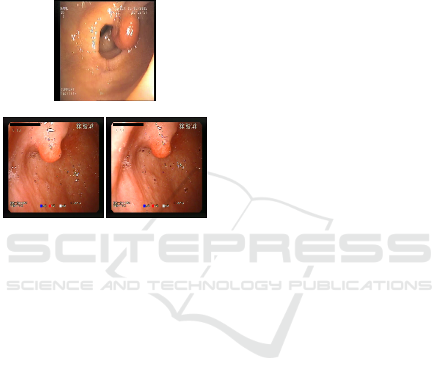
Figure 2 presents other image examples from this

dataset. The numbers in the upper left corner indicate

the frame number from the respective exam video.

The marked region shows the location of the anomaly

contained in the image. The colour of numbers and

markings indicate whether annotations are “Precise”

or “Imprecise”. Precise marks (in yellow, at frames

116, 12, and 180) were annotated by experts. The

Imprecise ones (in blue, composed of the remaining

frames) were deﬁned using the neighbouring frames

to those marked by experts, in which the authors per-

formed a visual analysis and adjusted the binary mask

to match the region of interest visually.

The dataset contains 115,429 images with labels

categorized as Imprecise, signiﬁcantly more than the

ICEIS 2024 - 26th International Conference on Enterprise Information Systems

532

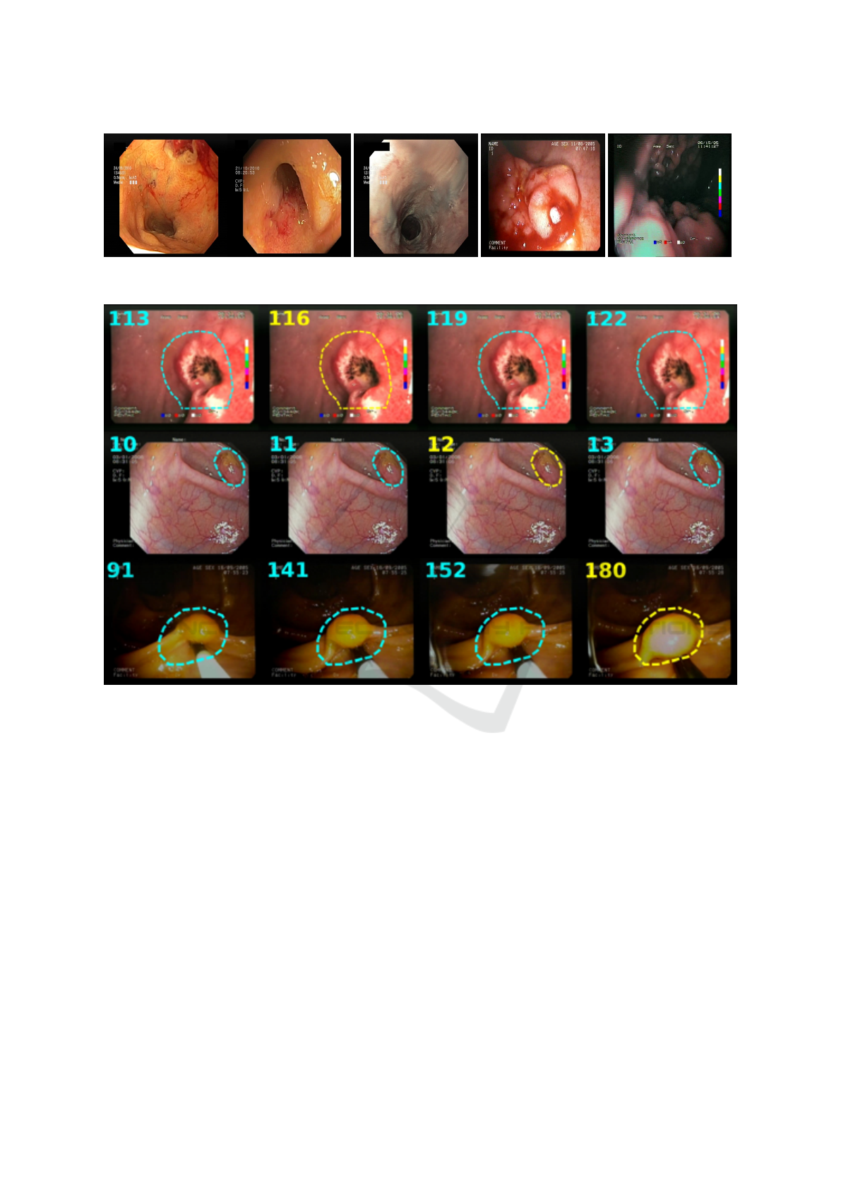
(a) Gastro. (b) Colono. (c) Healthy. (d) Blood. (e) Quality.

Figure 1: Examples of each category from ERS.

Figure 2: Example of images contained in the ERS dataset (Cychnerski et al., 2022).

number of images labelled by experts. Due to their

high abundance, however, imprecise images can be

instrumental in the training process of a deep learning

model, even with lower label accuracy. Furthermore,

the dataset has 866,612 images without any annota-

tions and 366,656 images from 7 WCE exams with

no labels.

In this dataset, images are split by patient, and

each patient can contain images from up to six differ-

ent exam videos. Each image may be associated with

0 or more labels (characterizing a multi-label dataset),

in addition to the possibility of having a binary mask

with the location of the ﬁnding for segmentation or

object detection applications. Finally, each image is

stored as a PNG ﬁle in the RGB colour space with an

original resolution of 720x576.

3.2 EfﬁcientNet

EfﬁcientNet is a family of CNN architectures pro-

posed by Tan and Le (Tan and Le, 2019), recog-

nized for its high performance in image classiﬁca-

tion challenges such as ImageNet and ImageNet-V2

(Recht et al., 2019). The authors developed these

architectures by combining coefﬁcients to scale the

network structure (the number of convolutional lay-

ers and their respective number of ﬁlters). This scal-

ing process, deﬁned as Compound Scaling, was done

through a heuristic method based on Grid Search,

which uniformly adjusts the width and depth of the

network structure and regulates the feature maps from

a ﬁxed set of scale coefﬁcients. Such coefﬁcients are

presented in the Equation 1:

A Comparative Analysis of EfﬁcientNet Architectures for Identifying Anomalies in Endoscopic Images

533







d = α

w = β

r = γ

(1)

Where:

• d: Depth;

• w: Width;

• r: Image resolution;

• φ: Coefﬁcient that represents the amount of avail-

able computational resources, deﬁned by the user;

The α, β, and γ coefﬁcients deﬁne how the re-

sources will be assigned in relation to depth, width,

and resolution, respectively. These coefﬁcients must

assume values greater than or equal to 1, subject to

the restriction presented in Equation 2:

α · β

· γ

≈ 2 (2)

These parameters can be estimated in 2 ways:

1. Assuming φ = 1 and estimating α, β and γ;

2. Assuming α, β and γ as constants and estimating

different values of φ.

The EfﬁcientNet family of networks was deﬁned

by this scaling method, being named from B0 to B7.

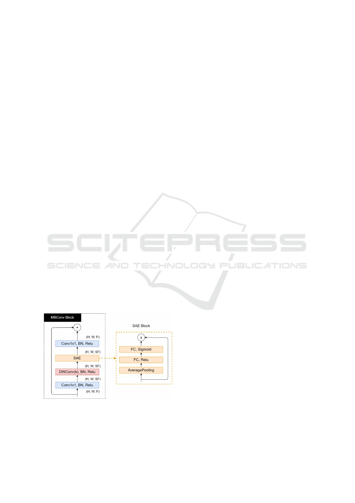
The structure of these networks is composed of blocks

called MBConv, being characterized by a combina-

tion between the Inverted BottleNecks (IB) (Sandler

et al., 2018) and the Squeeze-and-Excitation (SAE)

blocks (Hu et al., 2018). The IBs use depth-wise con-

volutions (DWConv) as alternatives to standard con-

volutions to reduce the computational cost of these

operations since DWConv operations have a smaller

amount of parameters to be adjusted (Howard et al.,

2017).

Figure 3: Structure of the MBConv and SAE blocks.

Figure 3 illustrates the structure of the MBConv

block and the SAE block. The input dimensions of

the MBConv blocks are H ×W × F, where H is the

height, W is the width, and F is the number of fea-

ture maps. More feature maps are generated after the

ﬁrst 1x1 convolution (followed by Batch Normaliza-

tion and a Relu activation). This increases by a scaling

factor S that multiplies F. Afterwards, the DWConv

operations are applied, generating another increase in

the number of feature maps, which will be used as

input to the SAE block.

The SAE blocks, illustrated in Figure 3, assign

weights to feature maps that are more relevant to the

model’s objective and will have greater weights. Fi-

nally, a last 1x1 convolution decreases the number of

feature maps, assuming its initial value.

In this work, these models were chosen because

they have comparatively lower computational costs

(requiring fewer FLOPS in the inference process and

with fewer adjustable parameters) and have better per-

formances considering the top-1 and top-5 accuracy

metrics in ImageNet (Recht et al., 2019), compared

to other well-known CNN architectures. The experi-

ments conducted in this work involving EfﬁcientNet

considered conﬁgurations from B0 to B3.

4 RESULTS AND DISCUSSION

4.1 Experiment Description

To conduct the experiments to evaluate the Efﬁcient-

Net architectures in the binary classiﬁcation of en-

doscopic images, the same approach as (Cychnerski

et al., 2022) was used to separate the images into

healthy and anomaly classes. In this approach, im-

ages were selected from the Healthy categories and

images without bleeding from the Blood category to

compose the set of healthy images, and images from

both the Gastro and Colono categories as well as

images with bleeding from the Blood category com-

posed the subset of images with pathologies.

A cross-validation method using ﬁve folds was

used. The folds were separated per patient to ensure

that exams from the same patient were not in separate

folds to avoid data leakage (Kaufman et al., 2012).

During each cross-validation stage, 20% of patients

from the training set were randomly selected for vali-

dation. As each patient has a different number of ex-

ams, the absolute number of images for each fold will

differ for each step. For the experiments, precise and

imprecise images were used to train and validate the

proposed models. For the evaluation, however, only

precise images were utilized.

Each model was trained for 25 epochs using Bi-

nary Cross-Entropy (Yi-de et al., 2004) as the loss

function, with the input resolutions ranging from

ICEIS 2024 - 26th International Conference on Enterprise Information Systems

534

224x224 to 300x300, depending on which model was

being trained. The network weights were initial-

ized with the pre-trained weights on ImageNet (Recht

et al., 2019), available through Keras (Chollet et al.,

2015).

To evaluate the performance of each trained

model, the Binary Accuracy value was used, as well

as the F1-Score metric. This metric represents the

harmonic mean of precision, the ratio of all true pos-

itives to all positive values returned, and sensitivity,

which represents the ratio of true positives returned to

all positive values present. This metric can be calcu-

lated as in Equation 3:

= 2

precision ∗ recall

precision + recall

2t p

2t p + f p + f n

(3)

With t p being the true positives, that is, the images

with correctly classiﬁed anomalies; f p being the false

positives, with the healthy images being incorrectly

classiﬁed; and f n being the false negatives, these be-

ing the images with anomalies classiﬁed as healthy.

values vary between 0 and 1, with higher values

indicating better results for the model.

The only work in the literature that can be com-

pared to the obtained results is (Cychnerski et al.,

2022), in which the ERS dataset was published. In

that work, the authors conducted some experiments

to serve as a baseline for comparison. In the case

of binary classiﬁcation, the authors tested several

deep neural network architectures, with MobileNet

v1 (Sandler et al., 2018) obtaining the best result.

The same cross-validation process was used for Mo-

bileNet v1, using the same ﬁve folds for a fair com-

parison.

4.2 Results

Table 1 compares the average results obtained with

MobileNetV1 and different EfﬁcientNet conﬁgura-

tions (B0-B3) using the same cross-validation method

and folds for each architecture. Each EfﬁcientNet

conﬁguration uses a different input image resolution

(as shown in the table), while the MobileNetV1 model

was trained with 240x240 resolution images. Notably,

all the different trained EfﬁcientNet conﬁgurations

obtained better results than the trained MobileNetV1

model, with differences of 8 to 15 percentage points

in the average Accuracy and 8 to 11 percentage points

in the average F1-Score. The standard deviation for

the Precision metric with MobileNet was also signiﬁ-

cantly higher, resulting in a higher standard deviation

for the F1-Score.

When analyzing the results between the Efﬁcient-

Net conﬁgurations, it is noticeable that the simplest

conﬁguration (B0 with the lowest resolution) obtained

better results than the others regarding almost all met-

rics, with differences varying between 2 and 3 per-

centage points considering the F1-Score (with practi-

cally the same standard deviation).

In Table 2, we have the results for each individ-

ual fold of the cross-validation using EfﬁcientNetB0,

which was the best-performing variation of the tested

architectures during the experiments. The Accuracy,

Precision, Recall, and F1-Score values for each test

fold and the mean and standard deviation for each in

this experiment are presented. The results are promis-

ing, reaching average values above 76% in all metrics.

However, the model’s difﬁculty in correctly classify-

ing healthy images is notable, as evidenced by the low

precision in fold 5, resulting in a relatively high stan-

dard deviation for this metric. This also resulted in

an accuracy value lower than the F1-Score achieved

due to more false positives and, consequently, a lower

number of true negatives (correctly classiﬁed healthy

images). However, the model performed better in cor-

rectly classifying images with anomalies, with F1-

Scores reaching 88.14% in fold 1 and obtaining an

average of 84.67%.

4.3 Case Study

Aiming to understand better the performance of Efﬁ-

cientNet in classifying images from the ERS dataset,

we selected the model that performed best during the

experiments (EfﬁcientNetB0 trained with folds 2-5)

and veriﬁed which images the model had the most

success and difﬁculties. To achieve this, we analyzed

the model outputs for the test set. We selected the im-

ages for which the model generated the highest and

lowest probabilities for correct and incorrect predic-

tions for both the positive and negative classes.

In Figure 4, we have examples of positive classi-

ﬁcations by the model. In Figure 4a and Figure 4c,

we have the predictions with the highest probability

for anomalies, for true positives and false positives,

respectively. Similarly, the lowest probability model

outputs for the positive class are presented in 4b and

4d. The positive case with the highest probability was

a polyp in the colon region. This was probably an

easy example of classiﬁcation for the model because

it was a frame with a very visually evident polyp. The

case of the correct positive prediction with the low-

est probability is an image of a duodenal ulcer. It is

noticeable that there are bubbles in the image in this

particular frame, which can complicate the model’s

inference process. However, it was still able to clas-

sify this example correctly.

Both examples of false positives are images of the

A Comparative Analysis of EfﬁcientNet Architectures for Identifying Anomalies in Endoscopic Images

535

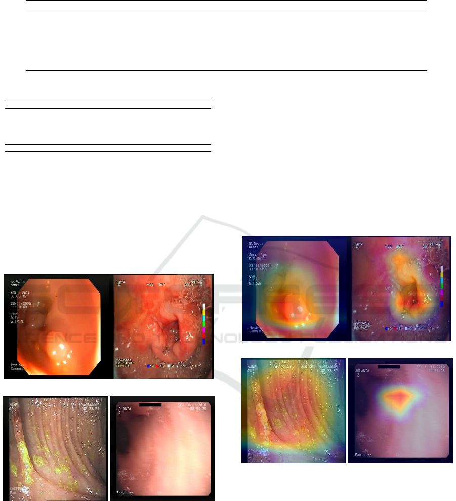
Table 1: Comparison between different EfﬁcientNet architectures and MobileNetV1.

Model Resolution Accuracy (%) Precision (%) Recall (%) F1-Score (%)

EfﬁcientNetB3 300x300 70.45 ± 4.64 69.84 ± 5.31 96.85 ± 0.94 81.04 ± 3.63

EfﬁcientNetB2 260x260 74.32 ± 5.44 75.04 ± 5.88 91.71 ± 3.44 82.40 ± 3.95

EfﬁcientNetB1 240x240 73.81 ± 5.62 74.38 ± 5.67 92.26 ± 2.63 82.23 ± 3.87

EfﬁcientNetB0 224x224 77.29 ± 5.44 76.52 ± 6.08 95.21 ± 1.42 84.67 ± 3.51

MobileNetV1 240x240 61.93 ± 6.41 66.88 ± 6.85 83.88 ± 15.78 73.55 ± 7.79

Table 2: Results for cross-validation with EfﬁcientNetB0.

Fold Acc (%) Precision (%) Recall (%) F1-Score (%)

Fold 1 84.46 81.95 95.35 88.14

Fold 2 78.19 78.90 95.78 86.53

Fold 3 74.05 74.07 94.98 83.23

Fold 4 80.86 81.89 92.78 87.00

Fold 5 68.89 65.78 97.17 78.45

Mean 77.29 ± 5.40 76.52 ± 6.08 95.21 ± 1.42 84.67 ± 3.51

colon region, even though most healthy images in this

dataset are from colonoscopies. The case in 4c prob-

ably resulted in a high probability for the class of

pathologies due to the yellow spots along the tract tis-

sue, which the model may have identiﬁed as features

of some anomaly. The image presented in 4d gen-

erated a false positive, possibly because it is a low-

quality image with some visual artifacts that could

have been confused with pathology features.

(a) Maximum true positive. (b) Minimum true positive.

Figure 4: Examples of predictions (correct and incorrect) as

pathologies.

To visualize the network’s decision process, the

Grad-CAM algorithm (Selvaraju et al., 2016) was

used to plot heatmaps that highlight the regions most

crucial for target class prediction. This algorithm was

applied to both the correct and incorrect cases pre-

sented previously to understand better the model’s

strengths and difﬁculties in detecting anomalies. Fig-

ure 5 shows the activation mappings of the last convo-

lutional layer of EfﬁcientNetB0 plotted over the cor-

responding images of the positive class. In 5a and 5b,

it can be seen that the emphasis is around the lesion

region, and in the case of 5b, little focus was given

to the area with bubbles. For the case in 5c, it can

be seen that the entire region with the yellow marks

was highlighted, so, in fact, this was mistaken for a

lesion. Finally, in 5d, it is noted that a small region

in the middle of the image has been highlighted, but

nothing particularly notable occurs in this location.

(a) Maximum true positive. (b) Minimum true positive.

Figure 5: Heatmaps mapping the activation for the positive

class.

Similarly to the previous ﬁgure, in Figure 6, we

have examples of the model’s negative classiﬁcations,

that is, predictions of healthy images. In 6a and 6b,

we have the frames that had the highest and lowest

probabilities for the negative class, respectively. This

probability was given as 1 − p, with p being the prob-

ability for the positive class. Both cases are from im-

ages of healthy tissue from the colon region. In con-

trast, the low probability of healthy tissue in Figure

ICEIS 2024 - 26th International Conference on Enterprise Information Systems

536

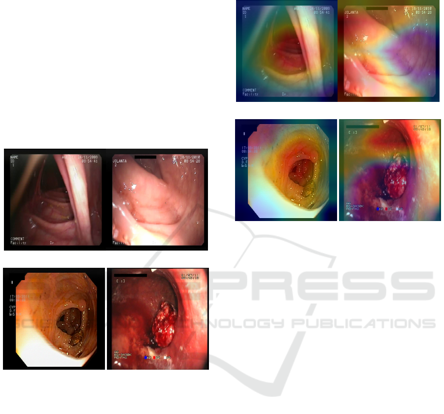
6b may be a consequence of the areas with high lu-

minosity in the lower part of the image. Figures 6c

and 6d, also parallel to the previous examples, are the

frames that had the highest and lowest probabilities

for the negative class, respectively, but were mistak-

enly classiﬁed as pathologies by the model. In Figure

6c, the model failed to recognize the region with a

polyp in the frame, probably attributing more signif-

icant importance to the areas of healthy tissue in the

image. In 6d, we have a severe case of false negative,

where the pathology is signiﬁcantly visually evident.

Still, the probability of the positive class did not ex-

ceed the classiﬁcation threshold and, therefore, was

erroneously classiﬁed as healthy.

(a) Maximum true negative. (b) Minimum true negative.

Figure 6: Examples of predictions (correct and incorrect) as

healthy images.

As was done for positive examples, the Grad-

CAM algorithm was also used to visualize the de-

cision process in the classiﬁcation examples for the

healthy class. To this end, the gradient of the out-

put of the network’s last convolutional layer was also

considered regarding the probability of the negative

class, that is, 1 − p, as previously described. Figure

7 presents the output of Grad-CAM for the presented

instances of classiﬁcations for the healthy class. In

7a, it can be seen that the activation for the healthy

class in this frame is in the center of the image, co-

inciding with the incidence of light from the colono-

scopic device and assigning less focus to the darker

parts of the image. Something similar happens in 7b,

and contrary to what was supposed, the regions with

the highest incidence of light were the most important

for the model’s decision in this classiﬁcation.

(a) Maximum true negative. (b) Minimum true negative.

Figure 7: Heatmaps mapping the activation for the negative

class.

For cases of incorrect classiﬁcations, 7c indicates

that the model assigned similar importance to a signif-

icant portion of the image, including the region con-

taining the polyp, pointing out that anomalies with

these features may be a weakness of this model. Fur-

thermore, the frame in 7d, despite pointing out that

little importance was given to the region where the

anomaly occurs for classiﬁcation as a healthy im-

age, the rest of the image had enough healthy tissue

features to warrant a negative classiﬁcation from the

model.

4.4 Impact of Mislabeling

Finally, when carefully checking the labels assigned

to the images used in the experiments, a problem was

noticed in the separation chosen for healthy images

and those with pathologies. In the same way as the

binary classiﬁcation experiments carried out in (Cy-

chnerski et al., 2022), images were selected from the

Healthy categories and images without bleeding from

the Blood category to compose the set of healthy im-

ages. However, it was noted that 3 images (frame 4

of patient 12, and frames 1 and 2 from patient 944, all

from the Precise subset) in the dataset were labelled

both as “No blood” and as an anomaly in the Gas-

tro or Colono category, which resulted in the same

image being labelled as both healthy and unhealthy.

Figure 8 shows the 3 frames where this occurred. The

A Comparative Analysis of EfﬁcientNet Architectures for Identifying Anomalies in Endoscopic Images

537

ﬁrst frame is a colonoscopy exam, while the last two

frames occur one after the other in another upper en-

doscopy exam. Interestingly, the three frames present

cases of polyps.

(a) Frame 4 of patient 12.

(b) Frame 1 of patient 944. (c) Frame 2 of patient 944.

Figure 8: Frames labelled both positive and negative.

The EfﬁcientNetB0 model trained with folds 2-5

of the cross-validation process presented previously

was also tested to evaluate the possible impact of this

mislabeling during the experiments. The probability

assigned to the positive class was veriﬁed. For the ﬁrst

image, a probability of 0.4656 was assigned, which

would result in a wrong classiﬁcation considering the

threshold of 0.5 used in this work. For the other

two images, the model assigned values of 0.6025 and

0.7797, respectively, correctly classifying the frames

as pathologies. It is assumed that these cases harmed

the learning of the model for pathology cases, in par-

ticular for polyp cases, even more so since the Keras

API dealt with the situation of the same instance with

multiple labels in a binary classiﬁcation, keeping the

last assigned label, which in turn was “healthy” for

the 3 frames.

5 CONCLUSIONS

Various diseases in the gastrointestinal tract can be

detected and prevented through CADe and CADx sys-

tems applied to endoscopic exam images. The au-

tomatic early identiﬁcation of pathologies present in

WCE exams can assist physicians in efﬁciently treat-

ing their patients. This work evaluated the perfor-

mance of networks from the EfﬁcientNet family of ar-

chitectures for binary classiﬁcation in WCE images.

The experiments were conducted using an extensive

dataset not used in the literature, and their results

were compared with the benchmark presented by the

dataset’s authors.

The results indicate that the simplest Efﬁcient-

Net conﬁgurations obtained better results for binary

classiﬁcation, but all the results were superior to the

best results obtained by the dataset authors. The val-

ues of the analyzed metrics indicate promising re-

sults for classifying anomalies in WCE images. Still,

it is essential to highlight that no studies involving

other possible tasks with this dataset, such as detect-

ing pathologies in images or multiclass classiﬁcation.

ACKNOWLEDGMENTS

The authors acknowledge the Coordenac¸

ao de

Aperfeic¸oamento de Pessoal de N

ıvel Superior

(CAPES), Brazil - Finance Code 001, Conselho

Nacional de Desenvolvimento Cient

ıﬁco e Tec-

nol

ogico (CNPq), Brazil, and Fundac¸

ao de Am-

paro

a Pesquisa Desenvolvimento Cient

ıﬁco e Tec-

nol

ogico do Maranh

ao (FAPEMA) (Brazil), Empresa

Brasileira de Servic¸os Hospitalares (Ebserh) Brazil

(Grant number 409593/2021-4) for the ﬁnancial sup-

port.

REFERENCES

Aabakken, L., Rembacken, B., LeMoine, O., Kuznetsov,

K., Rey, J.-F., R

osch, T., Eisen, G., Cotton, P., and

Fujino, M. (2009). Minimal standard terminology

for gastrointestinal endoscopy–mst 3.0. Endoscopy,

41(08):727–728.

Bao, G., Pahlavan, K., and Mi, L. (2015). Hybrid localiza-

tion of microrobotic endoscopic capsule inside small

intestine by data fusion of vision and rf sensors. IEEE

Sensors Journal, 15(5):2669–2678.

Blokus, A., Brzeski, A., Cychnerski, J., Dziubich, T.,

and Je¸drzejewski, M. (2012). Real-time gastroin-

testinal tract video analysis on a cluster supercom-

puter. In Zamojski, W., Mazurkiewicz, J., Sugier, J.,

Walkowiak, T., and Kacprzyk, J., editors, Complex

Systems and Dependability, pages 55–68, Berlin, Hei-

delberg. Springer Berlin Heidelberg.

Brzeski, A., Dziubich, T., and Krawczyk, H. (2023). Visual

features for improving endoscopic bleeding detection

using convolutional neural networks. Sensors, 23(24).

Chollet, F. et al. (2015). Keras. https://keras.io.

Cychnerski, J., Dziubich, T., and Brzeski, A. (2022). ERS:

a novel comprehensive endoscopy image dataset for

ICEIS 2024 - 26th International Conference on Enterprise Information Systems

538

machine learning, compliant with the MST 3.0 speci-

ﬁcation. CoRR, abs/2201.08746.

Dosovitskiy, A., Beyer, L., Kolesnikov, A., Weissenborn,

D., Zhai, X., Unterthiner, T., Dehghani, M., Min-

derer, M., Heigold, G., Gelly, S., Uszkoreit, J., and

Houlsby, N. (2020). An image is worth 16x16 words:

Transformers for image recognition at scale. CoRR,

abs/2010.11929.

Fonseca, F., Nunes, B., Salgado, M., and Cunha, A. (2022).

Abnormality classiﬁcation in small datasets of cap-

sule endoscopy images. Procedia Computer Science,

196:469–476. International Conference on ENTER-

prise Information Systems / ProjMAN - International

Conference on Project MANagement / HCist - Inter-

national Conference on Health and Social Care Infor-

mation Systems and Technologies 2021.

Goel, N., Kaur, S., Gunjan, D., and Mahapatra, S. (2022).

Dilated cnn for abnormality detection in wireless cap-

sule endoscopy images. Soft Computing, pages 1–17.

He, K., Zhang, X., Ren, S., and Sun, J. (2016). Deep resid-

ual learning for image recognition. In Proceedings of

the IEEE Conference on Computer Vision and Pattern

Recognition (CVPR).

Hewett, D. G., Kahi, C. J., and Rex, D. K. (2010). Ef-

ﬁcacy and effectiveness of colonoscopy: how do we

bridge the gap? Gastrointestinal Endoscopy Clinics,

20(4):673–684.

Howard, A. G., Zhu, M., Chen, B., Kalenichenko, D.,

Wang, W., Weyand, T., Andreetto, M., and Adam,

H. (2017). Mobilenets: Efﬁcient convolutional neu-

ral networks for mobile vision applications. CoRR,

abs/1704.04861.

Hu, J., Shen, L., and Sun, G. (2018). Squeeze-and-

excitation networks. In Proceedings of the IEEE Con-

ference on Computer Vision and Pattern Recognition

(CVPR).

IARC/WHO (2022a). Cancer Today - Brazil Fact Sheet.

https://gco.iarc.who.int/media/globocan/factshee

ts/populations/76-brazil-fact-sheet.pdf. Accessed:

13/02/2024.

IARC/WHO (2022b). Cancer Today - World Fact Sheet.

https://gco.iarc.who.int/media/globocan/factsheets

/populations/900- world-fact-sheet.pdf. Accessed:

13/02/2024.

Kaufman, S., Rosset, S., Perlich, C., and Stitelman, O.

(2012). Leakage in data mining: Formulation, de-

tection, and avoidance. ACM Trans. Knowl. Discov.

Data, 6(4).

Kavic, S. M. and Basson, M. D. (2001). Complications

of endoscopy. The American Journal of Surgery,

181(4):319–332.

Li, K., Wu, Z., Peng, K.-C., Ernst, J., and Fu, Y. (2018).

Tell me where to look: Guided attention inference

network. In Proceedings of the IEEE Conference on

Computer Vision and Pattern Recognition (CVPR).

Lin, K., Yang, H.-F., Hsiao, J.-H., and Chen, C.-S. (2015).

Deep learning of binary hash codes for fast image

retrieval. In Proceedings of the IEEE Conference

on Computer Vision and Pattern Recognition (CVPR)

Workshops.

Litjens, G., Kooi, T., Bejnordi, B. E., Setio, A. A. A.,

Ciompi, F., Ghafoorian, M., van der Laak, J. A., van

Ginneken, B., and S

anchez, C. I. (2017). A survey

on deep learning in medical image analysis. Medical

Image Analysis, 42:60–88.

Ma, L., Su, X., Ma, L., Gao, X., and Sun, M. (2023).

Deep learning for classiﬁcation and localization of

early gastric cancer in endoscopic images. Biomed-

ical Signal Processing and Control, 79:104200.

Muruganantham, P. and Balakrishnan, S. M. (2022). At-

tention aware deep learning model for wireless cap-

sule endoscopy lesion classiﬁcation and localiza-

tion. Journal of Medical and Biological Engineering,

42(2):157–168.

Ramsoekh, D., Haringsma, J., Poley, J. W., van Putten,

P., van Dekken, H., Steyerberg, E. W., van Leerdam,

M. E., and Kuipers, E. J. (2010). A back-to-back com-

parison of white light video endoscopy with autoﬂu-

orescence endoscopy for adenoma detection in high-

risk subjects. Gut, 59(6):785–793.

Recht, B., Roelofs, R., Schmidt, L., and Shankar, V. (2019).

Do ImageNet classiﬁers generalize to ImageNet? In

Chaudhuri, K. and Salakhutdinov, R., editors, Pro-

ceedings of the 36th International Conference on Ma-

chine Learning, volume 97 of Proceedings of Machine

Learning Research, pages 5389–5400. PMLR.

Sandler, M., Howard, A., Zhu, M., Zhmoginov, A., and

Chen, L.-C. (2018). Mobilenetv2: Inverted residu-

als and linear bottlenecks. In Proceedings of the IEEE

Conference on Computer Vision and Pattern Recogni-

tion (CVPR).

Selvaraju, R. R., Das, A., Vedantam, R., Cogswell, M.,

Parikh, D., and Batra, D. (2016). Grad-cam: Why

did you say that? visual explanations from deep

networks via gradient-based localization. CoRR,

abs/1610.02391.

Siegel, R. L., Miller, K. D., Goding Sauer, A., Fedewa,

S. A., Butterly, L. F., Anderson, J. C., Cercek, A.,

Smith, R. A., and Jemal, A. (2020). Colorectal cancer

statistics, 2020. CA: A Cancer Journal for Clinicians,

70(3):145–164.

Simonyan, K. and Zisserman, A. (2014). Very deep con-

volutional networks for large-scale image recognition.

arXiv preprint arXiv:1409.1556.

Szegedy, C., Vanhoucke, V., Ioffe, S., Shlens, J., and Wo-

jna, Z. (2016). Rethinking the inception architecture

for computer vision. In Proceedings of the IEEE Con-

ference on Computer Vision and Pattern Recognition

(CVPR).

Tan, M. and Le, Q. (2019). EfﬁcientNet: Rethinking model

scaling for convolutional neural networks. In Chaud-

huri, K. and Salakhutdinov, R., editors, Proceedings of

the 36th International Conference on Machine Learn-

ing, volume 97 of Proceedings of Machine Learning

Research, pages 6105–6114. PMLR.

Xie, E., Wang, W., Yu, Z., Anandkumar, A., Alvarez, J. M.,

and Luo, P. (2021). Segformer: Simple and efﬁcient

design for semantic segmentation with transformers.

In Ranzato, M., Beygelzimer, A., Dauphin, Y., Liang,

P., and Vaughan, J. W., editors, Advances in Neural

A Comparative Analysis of EfﬁcientNet Architectures for Identifying Anomalies in Endoscopic Images

539

Information Processing Systems, volume 34, pages

12077–12090. Curran Associates, Inc.

Yeung, M., Sala, E., Sch

onlieb, C.-B., and Rundo, L.

(2021). Focus u-net: A novel dual attention-gated cnn

for polyp segmentation during colonoscopy. Comput-

ers in Biology and Medicine, 137:104815.

Yi-de, M., Qing, L., and Zhi-bai, Q. (2004). Automated im-

age segmentation using improved pcnn model based

on cross-entropy. In Proceedings of 2004 Interna-

tional Symposium on Intelligent Multimedia, Video

and Speech Processing, 2004., pages 743–746.

Yu, X., Tang, S., Cheang, C. F., Yu, H. H., and Choi, I. C.

(2022). Multi-task model for esophageal lesion anal-

ysis using endoscopic images: Classiﬁcation with im-

age retrieval and segmentation with attention. Sen-

sors, 22(1).

Zhuang, H., Zhang, J., and Liao, F. (2021). A systematic re-

view on application of deep learning in digestive sys-

tem image processing. The Visual Computer, pages

1–16.

ICEIS 2024 - 26th International Conference on Enterprise Information Systems

540