Privacy Sensitive Building Monitoring Through Generative Sensors

Angan Mitra

, Denis Trystram

and Christopher Cerin

University of Grenoble Alpes, France

Keywords:

Smart Buildings, Sensor Combinatorial Optimization Problem in IoT, Ecological Sustainability,

Evolutionary Computing, Recommender Systems and Location-Awareness, Data Analytics.

Abstract:

A building equipped with sensors collects heterogeneous data, distributed naturally across zones. The lack

of spatiotemporal awareness can lead to excessive sensors or non-optimal distribution across a building. We

introduce a novel approach to reduce the friction between high smartness cost and ecological sustainability

by proposing virtual sensors as an artifact to estimate the environmental beneﬁt for the planet of doing the

”same with less.” The key idea behind the contribution is to inject data from virtual sensors to determine if

an actual sensor can be replaced, followed by a sub-grouping of sensors. As a ﬁrst contribution, our work

exploits the concept of ”less is more” to bring down the capital investment (CAPEX) and recurring expense

(OPEX) of the smart-building solutions. This fact opens the door to new research for an eco-responsible

deployment of sensors by revisiting the current approach of blind systematic deployment of sensors. We aim

to deploy the necessary amount (according to actual, simulated, or virtual uses) and not every room with all

possible sensors. As a second contribution, our experiments show a trade-off between virtualization accuracy

and active monitoring. Additionally, we validate our insights with 40-60% savings on sensor reduction for a

7-storied Thailand building.

1 INTRODUCTION

1.1 Context

The know-how of designing and making buildings

has seen tumultuous scales of updates, from huts to

skyscrapers. Before electricity advent, buildings were

conceived as a mere brick-and-mortar rendition of

habitable and workable spaces. When electrical ap-

pliances started populating households, the notion of

passive space turned into a controllable environment

using sensors and actuators. However, most of the ex-

isting buildings were already constructed before the

apparition of the Internet and the World Wide Web in

1990. This observation means building architectures

were not developed according to the sensors’ quantity,

type, and location.

Firstly, the popularity of Internet of Things (IoT)

devices led to ad-hoc dissemination in buildings,

where environments of dynamic parameters like tem-

perature, CO2, wind, etc., characterize buildings.

Such an approach can lead to a naive zonal distribu-

https://orcid.org/0000-0002-4581-808X

https://orcid.org/0000-0002-2623-6922

https://orcid.org/0000-0003-0993-9826

tion of sensors due to the obscurity of spatiotemporal

importance.

Secondly, a streaming IoT sensor can act as a data

source of sensitive patterns raising privacy concerns

among stakeholders.

Thirdly, the cost of equipping spaces with embed-

ded hardware over a large commercial area is non-

negligible and comes with recurring payments for

powering up the solution. In this work, we investigate

if there is a way to determine a minimalist sensing

solution for non-intrusive spatiotemporal coverage to

lower the capital cost and energy footprint of a smart

building solution.

In the realm of smart buildings, the convergence

of sensor combinatorial optimization problems within

the Internet of Things (IoT) landscape presents a sig-

niﬁcant opportunity for advancing ecological sustain-

ability. Through the lens of evolutionary computing,

complex algorithms can be harnessed to optimize sen-

sor placement, maximizing efﬁciency while minimiz-

ing environmental impact.

This approach not only enhances the functionality

of IoT systems but also aligns with principles of eco-

logical responsibility. Leveraging recommender sys-

tems and location-awareness technology further re-

Mitra, A., Trystram, D. and Cerin, C.

Privacy Sensitive Building Monitoring Through Generative Sensors.

DOI: 10.5220/0012728100003705

Paper published under CC license (CC BY-NC-ND 4.0)

In Proceedings of the 9th International Conference on Internet of Things, Big Data and Security (IoTBDS 2024), pages 107-118

ISBN: 978-989-758-699-6; ISSN: 2184-4976

107

ﬁnes data collection processes, ensuring that insights

derived from data analytics are both relevant and ac-

tionable.

However, amidst these advancements, the

paramount concern remains privacy-sensitive build-

ing monitoring. By integrating generative sensors,

which prioritize data anonymization and encryption,

the integrity of individual privacy is preserved

without compromising the efﬁcacy of smart building

operations. Thus, this holistic approach fosters

a symbiotic relationship between technological

innovation and ethical considerations, laying the

foundation for a sustainable and privacy-respecting

built environment.

1.2 Problem Statement and Outline of

Contributions

Given a temporal stream of data produced by IoT

sensors, we investigate the question of what subset

of sensors can be reliably powered off. We propose

a methodology for pre-integration and plan to place

sensors optimally within a building. The methodol-

ogy considers both virtual sensors (avatars) and non-

virtual sensors. The motivation for a virtual avatar

envelope over sensors in a building improves non-

intrusive sensing and reduces capital and operational

costs. The idea of an avatar to simulate a more ex-

tensive IoT infrastructure than the current one is one

of the main lines of our proposal. Since the markets

for smart buildings

and IoT

are overgrowing, it is

urgent to take into account as soon as possible, in

an eco-design approach, the need for a reasoned ap-

proach to the digitization of buildings.

In Section 2 we introduce the related works. In

Section 3 we propose a method to discover a logical

grouping of sensors at the edge and formulate encod-

ings to orchestrate a data-sharing policy. We solve

the underlying problem using a multi-objective opti-

mization algorithm to locate the edge network struc-

tures and identify distinct semantic collections. As

per experiments in Section 5, we empirically analyze

the policy evidence, discovery, and the lifelong mech-

anism of checking for optimal data-sharing topolo-

gies at the edge. Finally, summarizing in Section 6,

we argue that, for environmental issues, it is better to

pre-calculate the number of sensors and then buy and

deploy them rather than purchasing and deploying an

overestimation of the number of sensors.

https://www.fortunebusinessinsights.com/industry-

reports/smart-building-market-101198

https://iot-analytics.com/number-connected-iot-

devices/

2 RELATED WORK

Historically, buildings were not designed to cater to

forms of ambient intelligence, instead somewhat opti-

mized spatially for acceptable levels of thermal com-

fort, indoor ventilation, and privacy. Over time, the

building became a composite of observable and con-

trollable elements. In this section, we highlight the

limitations of the current situation in mastering the

placement of sensors, both at the technology level,

model level, and assumption level. Then we con-

duct a literature survey of the domain, such as sen-

sor approximation and optimal sensor placement. We

also introduce the machine learning and combinato-

rial optimization problem-solving concepts used in

our work.

2.1 Smart Building Technology

Acceptance

Smart applications (Wong et al., 2005) for buildings

have been developed mainly for monitoring, analysis,

and control of thermal units like Heating Ventilation

Air Conditioning (HVAC) units, illumination chan-

nels, etc. A 2019 review (Jia et al., 2019) of the smart

building industry states the major pain points towards

technological adaption. High installation costs, ob-

scurity on data storage policies, and privacy concerns

impede the acceptance (Hojjati and Khodakarami,

2016) of the Internet of Things in buildings. Typically

smart building applications thrive on real-time sensor

data for monitoring or actuation. Research shows that

analyzing sensor streams can reveal sensitive patterns

about occupancy (Garg and Bansal, 2000) or usage.

Consequently, privacy becomes a signiﬁcant concern

for occupants in a building due to the non-zero pos-

sibility of a data leak. The cost of constructing (Ma

et al., 2017) a smart building is usually 1.2-1.8 times

a non-smart counterpart. This initial capital poses the

second barrier for a stakeholder (Xu et al., 2019) to

overcome before system installation. But before a

technical deployment (Ma et al., 2016), the smart so-

lution needs to go through a pre-evaluation stage be-

fore ﬁnalizing the bill of materials.

2.2 Edge Learning for Smart Buildings

The incorporation of the Internet of Things (IoT) has

shaped machine learning-driven outcomes for predic-

tive maintenance, anomaly detection, resource opti-

mization, and much more. Sustainability goals have

put the spotlight on optimization possibilities for ex-

ploring frugality in the training of models (Gong

et al., 2021), inference on physical devices, etc.

IoTBDS 2024 - 9th International Conference on Internet of Things, Big Data and Security

108

The vision to enable battery-less computing (Nirjon,

2018) for platforms is shown to be capable of run-

ning predeﬁned machine learning tasks via intermit-

tent learning. Usually in the domain of IoT, the data

is on the move either between the cluster of devices

or to and fro from remote servers. Long-distance in-

formation propagation is energy-intensive for which

edge computing is growing to be a sustainable com-

puting partner for IoT.

Algorithmic developments and localized data han-

dling techniques at edge (Medeiros and Fernandes,

2020) to develop distributed learning models align

with a system-oriented approach (Thrun, 1995) to-

wards machine learning where one focuses on knowl-

edge representation and inferring meaningful infor-

mation against a stream of productive tasks (Chen and

Liu, 2016). Notably for buildings, the generated data

contains sensitive information regarding activity pat-

terns and this makes data sharing difﬁcult. This opens

the scope for federated learning (Mitra et al., 2021) or

decentralized techniques (Mitra et al., 2022) to pro-

mote building intelligence by strictly adhering to in-

house data policy. This line of work provides critical

insight into the role of communication topology and

utilization on a real-life smart building data set.

2.3 Sensor Allocation Problem

Multiple cyber-physical systems like sensors and ac-

tuators work in cohesion to maintain the desired qual-

ity of ambiance and indoor comfort of a building.

Some examples of non-intrusive ambient sensors are

temperature, humidity, and luminosity. Data val-

ues recorded by a type of sensor are usually dissim-

ilar across different buildings or separate zones in

a building. Empirical Mode Decomposition (EMD)

(Fontugne et al., 2012) of a continuous variable such

as temperature, humidity, or luminosity yields Intrin-

sic Mode Functions (IMF)(Ayenu-Prah and Attoh-

Okine, 2010). This model has been helpful for struc-

tural health monitoring (Barbosh et al., 2020) for

buildings. K means clustering over the space of IMF

for all the sensors is shown to be effective (Hong et al.,

2013) in identifying non-identical sensors. This ap-

proach is further extended (Yoganathan et al., 2018)

by using information loss to eliminate weak candidate

points from a cluster to obtain a sensor placement so-

lution.

Generally, choosing the globally optimal place-

ment within the search space of a large-scale com-

plex system is an intractable computation, in which

the number of possible placements grows combinato-

rially with the number of candidates (Ko et al., 1995).

Py-Sensors (de Silva et al., 2021) is a software pack-

age published in 2021 that includes state-of-the-art

algorithms on scalable optimization of sensor place-

ment from data. It is to be noted that the basis on

which one represents measurement data can have a

pronounced effect (Manohar et al., 2018) on the sen-

sors that are selected and the quality of the reconstruc-

tion. The task of classifying sites for sensor place-

ment for benchmarking is the Sparse Sensor Place-

ment Optimization for Classiﬁcation (SSPOC) algo-

rithm (Brunton et al., 2013). The algorithm is related

to compressed sensing optimization (Emmanuel et al.,

2005) but identiﬁes the sparsest set of sensors that

reconstructs a discriminating plane in a feature sub-

space. Regarding reconstruction problems, the pack-

age implements methods for efﬁciently analyzing the

effects that data or sensor quantity have on recon-

struction performance (Manohar et al., 2018). Of-

ten different sensor locations impose variable costs,

which are taken into account during sensor selec-

tion via a built-in cost-sensitive optimization routine

(Clark et al., 2018). Above mentioned methods are

neither incremental nor self-aware to attempt correc-

tive measures. Hence it is obscure how they will de-

tect changes in building patterns and correspondingly

adjust the sensor allocation/placements.

3 PROBLEM MODELING

The question ”How many are too few or too many

sensors” is often an undermined topic when installing

sensors in a building or multiple spaces. The work ad-

dresses data privacy for smart buildings and proposes

in-house data circulation as a backbone to power off

redundant sensors. In this context, we introduce the

Virtual Sensor Field, a mixed basket of physical and

computable sensors that creates a virtual avatar over a

set of sensors distributed over multiple spaces.

Figure 1 represents a high-level overview of the

virtual ﬁeld. The principal idea is grouping the set of

sensors the formulation is twofold:

1. Learn a methodology to partition the sensor set

S and provide insight on which sensors are most

likely to stay active or be replaced by virtual coun-

terparts.

2. Figure out how grouping sensors can leverage

data proximity at the edge, following a strictly in-

house data retention policy.

Assume that the notation n

means the number

of elements in set X. So in a building let there be n

sensors of n

types distributed over n

ﬂoors. Let

G be a collection of n

groups/sets, where for each

group g, active and virtual sensors are denoted by A

Privacy Sensitive Building Monitoring Through Generative Sensors

109

SENSOR

LOCATION MAP

ACTIVE SENSORS

VIRTUAL

SENSORS

HYPOTHESIS

SPACE

DRIFT AWARENESS (O

)

LEARN DATA CIRCULATION PROTOCOL (O

)

VIRTUAL TO REALITY

TRANSFORMATION (O

)

VIRTUAL FIELD

OPTIMIZATION

PATHWAY S

REALITY TO VIRTUAL

TRANSFORMATION (O

)

Figure 1: Schematic of Virtual Sensor Field with optimiza-

tion pathways.

and V

respectively.

|{z}

All Sensors

g=n

[

g=1

|{z}

Sensors in group g

(1)

|{z}

Group g Sensors

= A

|{z}

Active Sensors

∪ V

|{z}

Virtual Sensors

(2)

Now we break down the virtualization process

into three steps as follows:

• Reconstruction of hidden sensor data from real

or virtual deployed sensors. (Section 3.1)

• Classifying sensors as real or virtual and ﬁxing

where the sensors are to be placed. (Section 3.2)

• Re-calibration of virtual sensor ﬁeld with an in-

cremental data feed from real sensors. (Section

3.3)

3.1 Regressing Signal Reconstruction

The signal reconstruction mechanism reconstructs

virtual sensor data from actual sensors and vice versa

by creating a set of machine-learned regressors. Since

this mechanism works for every group before opti-

mization, one faces the cold start problem where the

optimal group size is unknown. Most importantly,

we bring to the reader’s attention that the classiﬁca-

tion for real and virtual sensors is a priori not known.

To resolve the issue, the system creates the following

seed groupings:

1. Bucketing sensors by the same type, thus ending

up with n

groups.

2. Grouping sensors by space or same ﬂoor, there-

fore creating n

groups.

Now for all of the cold start groups, the system

learns all possible pairwise regressors between sen-

sors. For example, in the case of spatial grouping,

the stream of a CO

type sensor can be reconstructed

using a luminous intensity sensor placed within the

same ﬂoor. Likewise, for a type-wise grouping, a tem-

perature sensor placed in the 2

ﬂoor can be approx-

imated using a similar type of candidate sensor from

the top ﬂoor. Thus, the learning complexity for n

logical groups is O(n

) models, where W is the

maximum group size.

The bidirectional transformation function be-

tween {A

, V

} is learned through per group hypoth-

esis space H

deﬁned by Equation 3.



: A

→ V

: V

→ A



(3)

refers to forward feature space that translates

from reality to the virtual world, while the subscript b

in H

denotes the reverse backward mapping between

hidden sensors and real-life deployment. The quality

of H

is evaluated through a cost function L (such as

Root Mean Square, L2, L1 norms) executed over all

possible pair-wise interaction pairs (u, v) ∀u ∈ S, v ∈

S, u ̸= v. The error in predicting channel v using a

sensor u is recorded at the [u, v]

index of an error

matrix E

as per Equation 4.

[u, v] = L(v, H

[u, v]

| {z }

ML model

(u)) (4)

Note that E

[u, v] ̸= E

[v, u] implies that the two

losses generated by swapping the dependent and in-

dependent variables may not be equal.

To estimate the sensor value y

of a channel v ∈

, we ﬁrst select the optimal channel (u

∗

) to predict

by using the [u

∗

, v]

entry of hypothesis library H

per Equation 5.

∗

← arg min

g∈G

[u, v]

= H

∗

, v](u

∗

)

(5)

This technique bounds the maximum observable

error since another optimal mapping H

∗

can exist us-

ing more than one feature for prediction.

3.2 Classifying Sensor Placement

Next, we introduce grouping sensors for answering:

How can we leverage intra-zone patterns to optimize

data ﬂows between sensors for virtualization? The

solution to such problems is typically a set of ’non-

dominated’ solutions where an objective can not be

improved without decreasing the other objectives. We

deﬁne the ﬁrst two objectives to measure the predic-

tion error due to forward H

and backward H

hy-

pothesis, respectively. For both equations 6 and 7,

symbols u and v shall stand for real and virtual sen-

sors, respectively.

(G)

| {z }

Virtual loss

= Σ

g∈G,u∈A

,v∈V

[u, v] (6)

IoTBDS 2024 - 9th International Conference on Internet of Things, Big Data and Security

110

(G)

| {z }

Inv Virtual loss

= Σ

g∈G,u∈A

,v∈V

[v, u] (7)

3.3 Re-Calibrating with Episodic Data

The system experimentally investigates the quality of

the sensor conﬁguration to power up the virtual sensor

ﬁeld optimally. Once optimal conﬁgurations are de-

ployed, valid sensor data at certain zones are missing.

Over time, predictions may lead to blind spots where

the ground truth may vastly deviate, or installing sen-

sors can become necessary.

Thus the afﬁnity grouping A

, V

can be re-

calibrated with the availability of additional data, but

such a process must consider the historical perfor-

mance. For any t ∈ T , reconstruction loss at sensor

position i is the absolute difference between the ac-

tual (y

) and predicted value ˆy

of a sensor for a virtual

mask is given as per Equation 8.

(G,t

)

| {z }

Reconstuction Feed

t∈[t

]

i∈S

−t

(t) − ˆy

(t)|

ˆy

(t) ∈

(

) i f s

∈ A



)) i f s

∈ V

(8)

3.4 Data Network Sparsity

The policymaker additionally models the network

topology of sensors to minimize the number of data-

sharing links. Let every node i have e

number of in-

coming edges and e

outgoing connections. Equation

9 gives O

deﬁned as the ratio between the number of

edges in M to the total edges in a complete graph. In a

spectral space spanned by n

entries, the representa-

tion for any sensor u is given by α

∈ R

and the net

non-randomness(O

) of the underlying connectivity

network is simply the sum of all possible pairwise dot

product between nodes.

(S)

|{z}

Networking Volume

= Σ

i∈S

+ e

(9)

The non-randomness of an edge tends to be small

when the two nodes linked by that edge are from

two different communities. The quality of the Vir-

tual Sensor Field is further tracked through a relative

measure that indicates to what extent the data shar-

ing/connectivity graph differs from random graphs in

terms of probability.

When O

is close to 0, the graph tends to be more

likely generated by an Erdos Renyi model.

4 SENSOR FIELD

VIRTUALIZATION SOLVER

We now present the solver that combines all 4 objec-

tives as formulated above, under Section 3 to optimize

the sensor placement incrementally. Each placement

strategy is encoded as a vector of numbers, and such a

vector shall be referred to as a policy. A policy assigns

a group number and a 0/1 tag indicating every sen-

sor’s virtual or physical presence. For example, if a

sensor belongs to group i, and has a virtualization tag

j ∈ {0, 1}, then the encoding is given as 2 × i + j. The

search space for all possible placements of n

sensors

is exponential in the order of 2

4.1 Policy Building Routine

Let P be a set of policies modeling non-identical sen-

sor placement conﬁgurations. How to cherry-pick ro-

bust positions and create partial ordering amongst

multiple strategies? Algorithm 1 creates an or-

dered front (φ) of positioning strategies which ac-

celerates decision-making. It uses non-dominated

sorting to obtain solutions superior to other conﬁg-

urations. This enables incrementally adding sensors

Pareto-optimally while keeping track of the number

of solutions inferior to a policy within the pool. The

candidate solutions with maximal superiority are in-

cluded in the ﬁrst front/batch to build up the sensor

blanket bottom-up.

4.2 Policy Exploration Routine

How to ascertain if there is a relative advantage in

switching from one conﬁguration to another? The an-

swer is a Gain Matrix (GN) of size M × N with M

policies and N objectives. The core intuition behind

Algorithm 2 is the density of solutions within a pol-

icy’s neighborhood. The policy pool is sorted for ev-

ery objective in ascending order, and the correspond-

ing objective weight initializes the starting objective

value for each sensor conﬁguration. Each element of

Gain Matrix GN is updated with the differential mar-

gin of the objective scores between the policies at the

i − 1 and i + 1 index. Note that if all the objectives’

values are co-linear, the gain term is 0.

Policy Explorer spans the conﬁguration space

through two well studied genetic operators (Um-

barkar and Sheth, 2015). Mutation operates per group

and randomly toggles a sensor from the active group

) to the virtual group (V

) and vice-versa. The

second operator, the Random Crossover, is performed

amongst two randomly chosen afﬁnity groups within

a policy mask.

Privacy Sensitive Building Monitoring Through Generative Sensors

111

Algorithm 1: Sensor Front Builder.

Input: Policy set P

Output: Ordered Sensor Front φ

1: for every policy p ∈ P do

2: for every policy q ∈ P do

3: if p ≻ q then

4: S

← S

∪ {q} { ▷ absorb policy q since

every objective in q is better than p }

5: else if q ≻ p then

6: n

= n

+1 { ▷ Count how many solutions

are superior in S to q. }

7: end if

8: end for

9: if n

=0 then

10: φ

= φ

∪ {p} { ▷ Select only non-

dominating solutions as the ﬁrst front. }

11: end if

12: end for

13: i= 1

14: while φ

̸= 0 do

15: C = φ { ▷ For every front, incrementally add

sensors starting from zero.}

16: for each p ∈ φ

17: for each q in S

18: n

= n

− 1

19: if n

= 0 then

20: C = C ∪ {q} { ▷ Add non-dominant

sensors to a placement conﬁguration}

21: end if

22: i = i + 1; φ

= C

23: end for

24: end for

25: end while

Algorithm 2: Differential Gain Estimator.

Input: Policy pool P of size M,

N objective functions

Output: Gain Matrix GN of size M × N

1: for every objective j ∈ 1 to N do

2: GN

[p] = O

(p)∀p ∈ P. { ▷ Number of entries

in GN

= M}

3: GN

[0] = GN

[M] = 0

4: for i = 2 to M − 1 do

5: GN

[i]+ = (GN

[i − 1] − GN

[i + 1])

6: end for

7: end for

4.3 Policy Optimizer Routine

In Algorithm 3 NSGA II (Deb et al., 2002) is mod-

iﬁed to search the conﬁguration vector space, with

time complexity of O(2

), to optimize our objectives,

Algorithm 3: Policy Optimizer.

Input: Initial policy pool P

t=0

of size M

N objective functions,

Iteration Limit T

max

Output: M best policies

1: Initialize t ← 0, Q

t=0

= φ

2: while t ≤ T

max

3: R

← P

∪ Q

4: φ = Sensor Front Builder(R

)

5: i ← 0 {▷ Incrementally add conﬁgurations}

6: while i < |φ| do

7: P

t+1

= P

∪ φ

8: GN ← Differential Gain Estimator(φ

)

9: Sort(P

t+1

) based on GN

10: P

t+1

= P

t+1

[1 : M] {▷ Get top M policies}

11: i ← i + 1

12: end while

13: Q

t+1

= Policy Explorer(P

t+1

)

14: t ← t + 1

15: end while

and as follows:

1. Take as input the learned hypothesis space and er-

ror matrix {H

, E

}∀g ∈ G.

2. Initialize a ﬁxed-sized sample pool (P

) of policies

as a random string of 0’s and 1’s.

3. For every policy, evaluate the objective set

, O

4. If the maximum number of generations is reached

or incremental gain is lower than a threshold, the

algorithm stops; else, a child population Q

is cre-

ated using steps 5, 6, and 7.

5. Policy sorting is used to incrementally identify

Pareto optimal solutions till the entire population

is exhausted.

6. Policy Gain Estimator is used to check the density

around individual solutions to prevent the algo-

rithm from terminating in a local optimum. Poli-

cies within the rectangular ﬁeld spanned by the

nearest adjacent solutions are discarded.

7. Alteration in the encoding is achieved through ge-

netic operators: Random Crossover (Umbarkar

and Sheth, 2015) implemented as the policy sam-

pler.

8. Finally populations P

and Q

are combined to

generate the parent population at time t + 1 using

steps 5 and 6 in order.

9. Go back to Step 3 and iterate with the generation

count decreased by 1.

IoTBDS 2024 - 9th International Conference on Internet of Things, Big Data and Security

112

5 EXPERIMENTS

5.1 Data Set, Settings and Experimental

Plan

We consider the dataset from (Pipattanasomporn

et al., 2020) for the experiments. It comes from a

seven-ﬂoor building in Thailand, including 24 smart

zones with 1.5 years of data collected at a 1-minute

resolution. The analysis highlights three key decom-

position steps to build up a Virtual Sensor Field:

• Evidence Investigation of error matrices ({E

})

to judge the quality of virtualization accuracy as

per sub-section 5.2.

• Policy Encoding (M) for generating a virtual sen-

sor ﬁeld according to sub-section 5.3.

• Policy Re-calibration to incrementally build up a

policy from the bottom up by optimizing the hy-

pothesis space as given in sub-section 5.4.

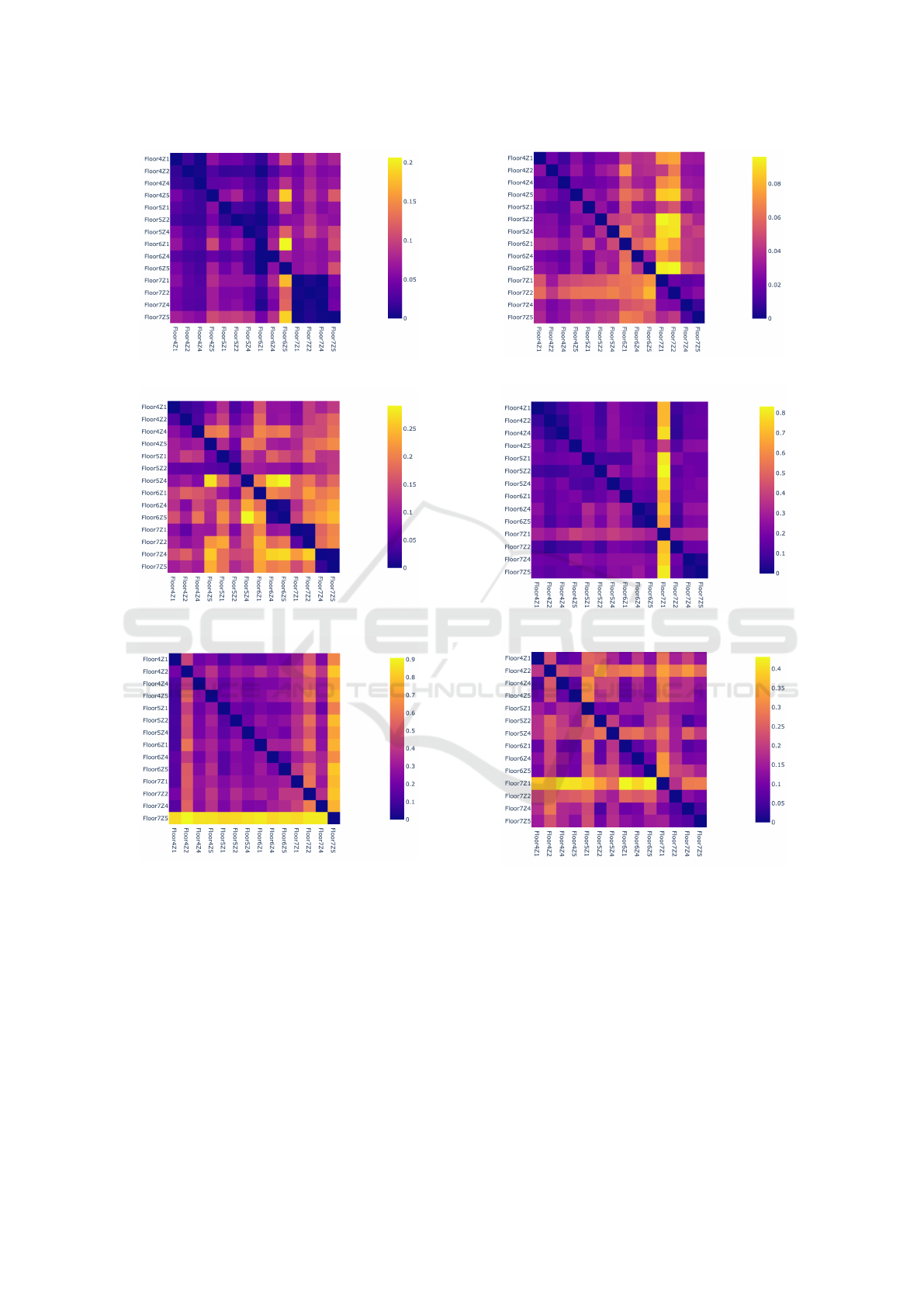
5.2 Evidence Investigation

Table 1: Error Matrix with Spatial Grouping when predict-

ing a sensor of type t and ﬂoor f, all the sensors from f are

used for forecasting.

Zone Power Ambience

AC Light App Temp RH Lux

FL-2Z1 0.15 0.14 0.13 0.18 0.53 0.15

FL-2Z2 0.08 0.07 0.15 0.11 0.36 0.06

FL-2Z4 0.33 0.31 0.73 0.33 0.66 0.31

FL-3Z1 0.32 0.23 0.38 0.24 0.45 0.26

FL-3Z2 0.35 0.25 0.27 0.29 0.4 0.27

FL-3Z4 0.34 0.23 0.25 0.22 0.61 0.22

FL-3Z5 0.42 0.25 0.27 0.28 0.63 0.24

FL-4Z1 0.28 0.24 0.19 0.2 0.53 0.26

FL-4Z2 0.34 0.27 0.48 0.25 0.59 0.25

FL-4Z4 0.28 0.25 0.29 0.24 0.53 0.24

FL-4Z5 0.36 0.18 0.35 0.23 0.46 0.17

FL-5Z1 0.23 0.2 0.19 0.15 0.45 0.22

FL-5Z2 0.29 0.19 0.28 0.19 0.35 0.19

FL-5Z4 0.33 0.36 0.31 0.3 0.58 0.3

FL-5Z5 0.43 0.26 0.29 0.31 0.64 0.26

FL-6Z1 0.26 0.23 0.25 0.29 0.37 0.22

FL-6Z2 0.36 0.28 0.22 0.28 0.38 0.3

FL-6Z4 0.26 0.17 0.27 0.22 0.41 0.21

FL-6Z5 0.47 0.22 0.26 0.23 0.58 0.23

FL-7Z1 0.34 0.28 0.43 0.31 0.65 0.48

FL-7Z2 0.31 0.3 0.59 0.33 0.61 0.23

FL-7Z4 0.28 0.21 0.28 0.23 0.41 0.2

FL-7Z5 0.44 0.38 0.71 0.34 0.61 0.36

What is the trade-off in terms of accuracy between

keeping a sensor powered on and alternately switched

off within a group g? Once a grouping strategy is

ﬁxed, the system trains a forecasting model between

two sensor channels (u,v) for every sensor map group

, V

). n

disjoint groups enable computing the

hypothesis space H

and the error matrix table in par-

allel. For every prediction task between u, v, the com-

puted center generates an error matrix for each model,

for example, linear regression, random forest, and

XGBoost. The training step ingests 90 days of sen-

sor data feed from every type of sensor in each place.

The evidence described corresponds to one month per

season train feed picking three months from each of

the:

• Summer (March - June). Hottest time of the year

with an average low of 25 degrees to an average

high of 35 degrees.

• Rainy Season (July – October). Average mini-

mum 24 degrees and average high 32 degrees.

• Winter (November – February). Average mini-

mum 20 degrees and average high 29 degrees.

Tables 1 reﬂect the maximum error recorded with

space-wise grouping, respectively. For every chan-

nel, the minimum and the maximum training errors

are presented as a tuple. Power consumption patterns

are best learned from a similar category of sensors

(min = 0.03, max = 0.27, grouping = type) rather than

combining data from multiple heterogeneous sensors

in the same place (min = 0.2, max = 0.71, grouping

= space). This observation is consistent for predicting

light, AC, and appliance power consumption levels as

seen from Figure 2.

Luminosity (lux) levels have the best type-wise

grouping approximation (min=0.03, max=0.14), al-

though, for ﬂoor 2 Zone 2, we observe spatial group-

ing lower error E (spatial) = 0.06 < E (domain) =

0.09. For indoor temperature prediction, domain-

wise grouping (min=0.04, max=0.14) yields an error

lower than (min=0.19, max=0.71, grouping = space)

for all ﬂoors except in ﬂoor 2 with zone 1, where Er-

ror (spatial) = 0.18 < Error (domain) = 0.25, and for

zone 2 Error (spatial) =0.11 < E (domain) = 0.24.

The relative humidity is most challenging to approx-

imate (min=0.37, max=0.66, grouping = space) and

(min=0.14, max=0.63, grouping = type) across all

zones. Overall we see that domain-wise grouping per-

forms better on average, which conﬁrms the intuitive-

ness of being guessed easily by similar peers as seen

from Figure 3.

5.3 Policy Discovery

The policy is a 1D vector made up of n

= 138 pos-

itive numbers where each integer encodes the data

afﬁnity group number and a Boolean instruction (0/1)

indicating whether to be powered off or on, respec-

Privacy Sensitive Building Monitoring Through Generative Sensors

113

(a) AC Power.

(b) Light Power.

Figure 2: Virtualization prediction on treating an identical

type of power meters as one group.

tively. Given an exhaustive set of policy evidence, the

task is to optimize the bi-partition of {A

, V

} for

every group g belonging to the afﬁnity mask (A). A

pool of 50 candidate policies is randomly generated

and acts as an input to Algorithm 3, optimized over

sensor groups.

Figure 4a displays the variation in reconstruction

loss O

on the test data when training the system

with only O

, O

losses and then additionally plug-

ging topology loss (O

). It is seen that the fraction of

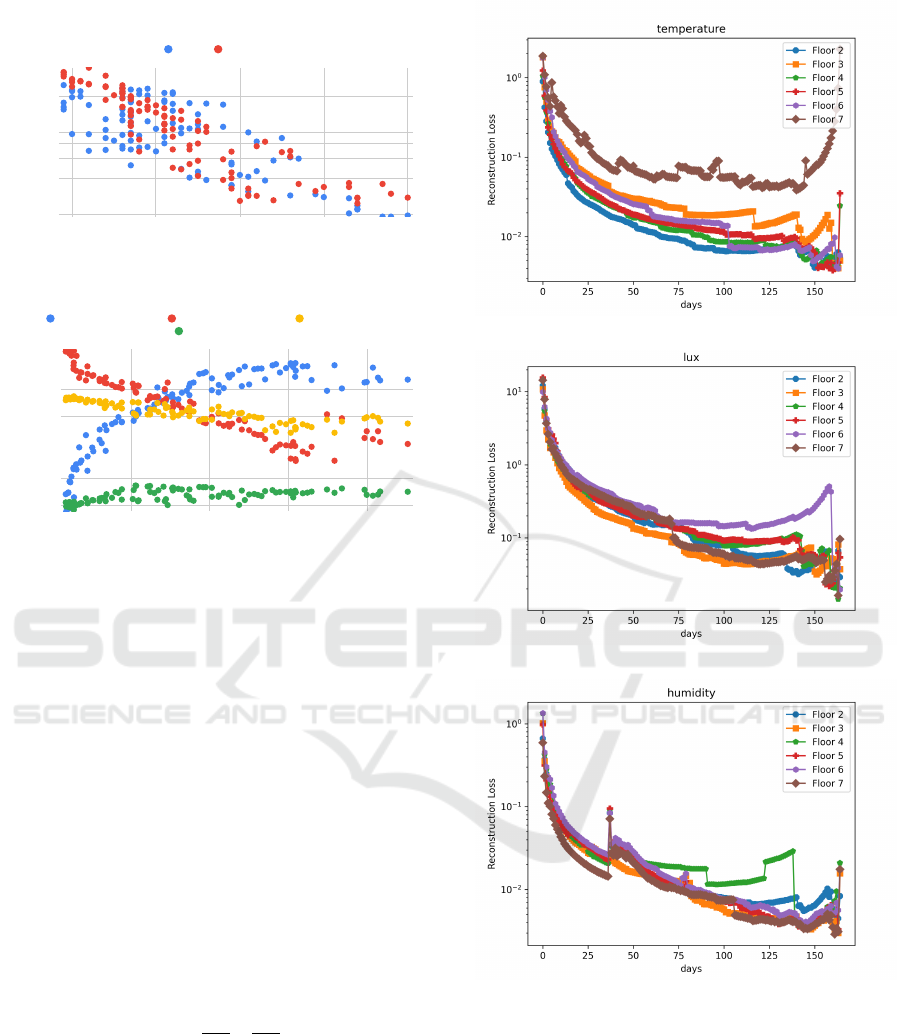
(a) Temperature.

(b) Luminosity.

Figure 3: Virtualization prediction on processing similar

ambiance channels as one group.

sensors bounded by the policy region of O

∈ (1, 2) ∧

∈ (0.5, 1) is around 45-65% and has a backward

translation error between (0.4, 1.2). Regarding O

from Figure 4b, it is observed that 5-10 % of total

possible edges or data ﬂow paths are sufﬁcient for a

policy to be competitively accurate. Indeed, policy

conﬁgurations exist where the observed error differ-

ence is bounded by within 1.5 units of deviance for

ambiance and energy monitoring sensor groups.

IoTBDS 2024 - 9th International Conference on Internet of Things, Big Data and Security

114

Number of Sensors

Reconstruction Loss(O3)

0.2

0.4

0.6

0.8

60 70 80 90 100

O1,O2 O1,O2,O4

Effect of objectives on Topology Discovery

(a) Discovering Policy Space.

Reconstruction Loss (O3)

Measurement Scale

0.05

0.1

0.5

1 2 3 4

Forward Translation (O1) Backward Translation (O2) Fraction of sensors

Sparseness (O4)

(b) Evaluating Objectives.

Figure 4: Characteristics of the Policy Space.

5.4 Policy Re-Calibration

This subsection answers how to incrementally build

up a policy mimicking the situation where a tempo-

rary sensor collects data and updates the policy on

the ﬂy. It is desired for a re-calibrated sensor place-

ment conﬁguration to have high conﬁdence in detect-

ing relatively more challenging spatiotemporal sen-

sor patterns. This helps in deciding which sensors

to include, thereby generating the most negligible re-

construction loss at run time. Once Pareto Optimal

Sensor conﬁgurations are generated using the train

data, the system tracks their performance over time

on the hold-out data, assuming every policy is exclu-

sively deployed. The data set per sensor be split into B

batches, where a batch i for a sensor k placed at zone

z is denoted by D

k,z

≡ [

max

+ B]. On receiv-

ing D

k,z

at i

time-step, the learning system evaluates

4 objectives denoted by Equations 6 - 8 to generate

better data transfer topologies. Figures 5 and 6 show

the reconstruction error O

on test year for each of 6

sensor types.

We discover that the temperature at the topmost

ﬂoor of the building is susceptible to the maximum

environmental ﬂuctuations, and expressed by the di-

verging nature of O

> 10% in Figure 5a. Some of the

(a) AC Power Prediction.

(b) Illumination Power Prediction.

Figure 5: Variation of reconstruction loss O

in ambiance

sensing group with increasing data feed (X-axis).

signiﬁcant factors that inﬂuence the luminosity level

at a spot are natural lighting, artiﬁcial illumination,

and occlusion. The interaction between the three el-

ements is more complicated to model than control-

ling the power for lighting. It is revealed by compar-

ing reconstruction loss (O

) between luminosity lev-

els and power consumption in Figures 5b and 6b, re-

spectively. Due to unknown spatial orientation, it is

Privacy Sensitive Building Monitoring Through Generative Sensors

115

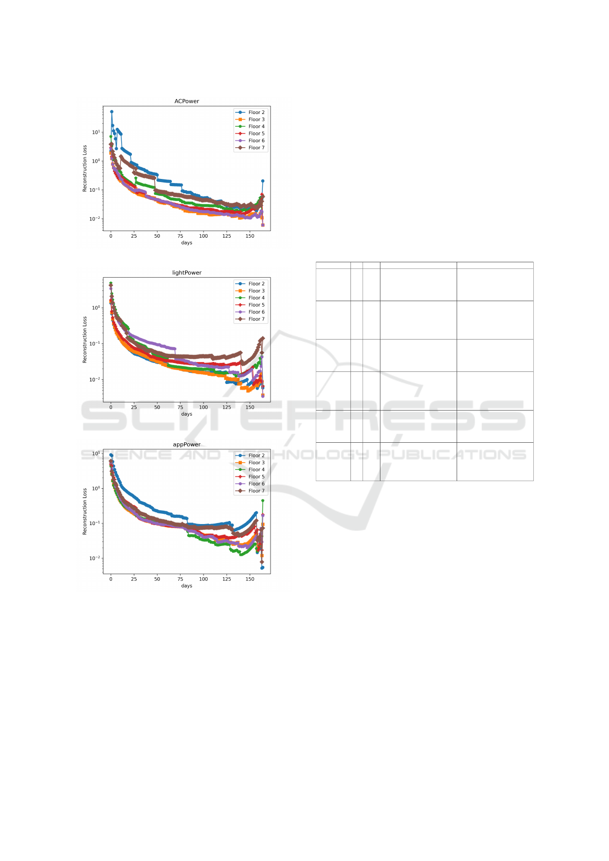
(a) AC Power Prediction.

(b) Illumination Power Prediction.

Figure 6: Variation of reconstruction loss O

in energy con-

sumption group with increasing data feed (X-axis).

hard to tell which zones have windows. On average,

the approximating power consumption shows close to

10 times lower reconstruction loss than ambient sen-

sors like temperature, luminosity, and humidity. As

per Figure 6a, 75 days or 2.5 months of data collec-

tion sufﬁces to keep the approximation error below

10% for all the six ﬂoors, the probable reason be-

ing controlled power consumption by an AC. Notably,

the approximation ability of light power and lux is

close to 98% accurate for ﬂoor 2 compared to 90%

correct for the top two ﬂoors (6,7). In a continual

setting, the system updates the hypothesis space and

auto-re-calibrates to stabler sensor placement conﬁg-

urations with the availability of more data. Table 2

gives the optimal sensor placement distribution that

uses 45 sensors instead of 138, bringing in a 67% sen-

sor reduction.

Table 2: Optimal installation suggestions to ecologically

monitor the seven-storied buildings in Thailand as covered

by the data set.

Type # Save Installation Sites Approximated Locations

Temperature 9 0.61

’FL-4Z4’, ’FL-2Z2’, ’FL-4Z2’,

’FL-3Z1’, ’FL-7Z5’, ’FL-3Z2’,

’FL-5Z1’, ’FL-7Z1’, ’FL-3Z5’

FL-4Z5’, ’FL-6Z4’, ’FL-6Z5’,

’FL-2Z1’, ’FL-6Z1’, ’FL-2Z4’,

’FL-6Z2’, ’FL-4Z1’, ’FL-7Z4’,

’FL-5Z5’, ’FL-5Z4’, ’FL-7Z2’,

’FL-3Z4’, ’FL-5Z2’

Humidity 6 0.74

’FL-4Z4’, ’FL-3Z1’, ’FL-7Z2’,

’FL-7Z1’, ’FL-3Z5’, ’FL-5Z2’

FL-4Z5’, ’FL-2Z2’, ’FL-6Z4’,

’FL-6Z5’, ’FL-2Z1’, ’FL-6Z1’,

’FL-4Z2’, ’FL-2Z4’, ’FL-6Z2’,

’FL-4Z1’, ’FL-7Z4’, ’FL-7Z5’,

’FL-5Z5’, ’FL-3Z2’, ’FL-5Z4’,

’FL-5Z1’, ’FL-3Z4’

Luminosity 8 0.65

’FL-2Z2’, ’FL-2Z1’, ’FL-6Z1’,

’FL-4Z2’, ’FL-3Z1’, ’FL-7Z5’,

’FL-3Z2’, ’FL-7Z2’

’FL-4Z5’, ’FL-4Z4’, ’FL-6Z4’,

’FL-6Z5’, ’FL-2Z4’, ’FL-6Z2’,

’FL-4Z1’, ’FL-7Z4’, ’FL-5Z5’,

’FL-5Z4’, ’FL-5Z1’, ’FL-7Z1’,

’FL-3Z5’, ’FL-3Z4’, ’FL-5Z2’

lightPower 7 0.7

’FL-2Z2’, ’FL-6Z5’, ’FL-4Z1’,

’FL-3Z1’, ’FL-7Z5’, ’FL-7Z2’,

’FL-3Z4’

’FL-4Z5’, ’FL-4Z4’, ’FL-6Z4’,

’FL-2Z1’, ’FL-6Z1’, ’FL-4Z2’,

’FL-2Z4’, ’FL-6Z2’, ’FL-7Z4’,

’FL-5Z5’, ’FL-3Z2’, ’FL-5Z4’,

’FL-5Z1’, ’FL-7Z1’, ’FL-3Z5’,

’FL-5Z2’

ACPower 10 0.57

’FL-2Z1’, ’FL-6Z1’, ’FL-7Z4’,

’FL-3Z1’, ’FL-7Z5’, ’FL-3Z2’,

’FL-5Z4’, ’FL-7Z2’, ’FL-5Z1’,

’FL-5Z2’

’FL-4Z5’, ’FL-4Z4’, ’FL-2Z2’,

’FL-6Z4’, ’FL-6Z5’, ’FL-4Z2’,

’FL-2Z4’, ’FL-6Z2’, ’FL-4Z1’,

’FL-5Z5’, ’FL-7Z1’, ’FL-3Z5’,

’FL-3Z4’

appPower 5 0.78

FL-4Z4’, ’FL-2Z4’, ’FL-4Z1’,

’FL-5Z4’, ’FL-5Z1’

’FL-4Z5’, ’FL-2Z2’, ’FL-6Z4’,

’FL-6Z5’, ’FL-2Z1’, ’FL-6Z1’,

’FL-4Z2’, ’FL-6Z2’, ’FL-7Z4’,

’FL-3Z1’, ’FL-7Z5’, ’FL-5Z5’,

’FL-3Z2’, ’FL-7Z2’, ’FL-7Z1’,

’FL-3Z5’, ’FL-3Z4’, ’FL-5Z2’

5.5 Comparative Study

Now we test the performance of the virtual sensing

ﬁeld in comparison to a random distribution, Sup-

port Vector Decomposition guided placement, and

sparse sensor placement optimization for classiﬁca-

tion (SSPOC) (de Silva et al., 2021). When the

number of sensors is gradually incremented, Figure

7 shows the performance gain in accuracy using our

approach. The benchmark methods show a low vir-

tualization quotient thereby needing more sensors to

maintain comparable levels of accuracy. The key

highlights of our approach to monitoring a building

are as follows:

• Evidence investigation measures the virtualiza-

tion capacity at every place and displays the error

if a sensor were to be powered off at that spot.

• Sensor placement conﬁguration is augmented

with in-house data circulation pathways. We ob-

IoTBDS 2024 - 9th International Conference on Internet of Things, Big Data and Security

116

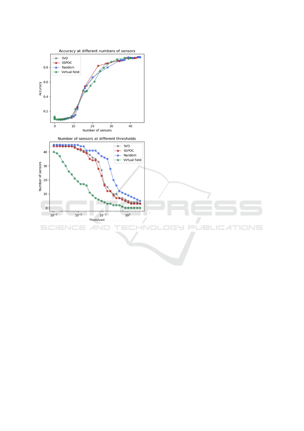
Figure 7: Gain in accuracy using virtual sensing ﬁeld in

comparison to state of art SSPOC and SVD methods.

serve the topological gain in obtaining a better

estimator through linking sensors of similar type

rather than constraining to ﬂoor-speciﬁc only.

• The system, in a nutshell, segregates sensor data

stream into more intricate and more straightfor-

ward predictable patterns. The procedure shows

a lifelong re-calibration strategy to afﬁrm the in-

tuition that placing sensors mostly at places with

low virtualization capacity can provide 100 %

coverage with less than 10 % error.

For example, the behavior of a group of tempera-

ture sensors situated across multiple zones can prob-

ably be learned by an optimal fraction of embedded

devices. For example, a sensor with a power rating of

50 watts consumes 0.05×365×24 = 438 units yearly.

Now imagine 100 such operating sensors, therefore

needing, 43, 800kW h of energy annually. One can ar-

gue about lowering the energy need by powering up a

fraction of the sensors only.

6 CONCLUSION

In this paper, we demonstrate that, according to a gen-

eral methodology, too many sensors are usually de-

ployed in buildings. Thus, this work emphasizes the

utility of spatiotemporal knowledge in bringing down

the operating cost of building management systems.

With explainable insights, the missing sensor approx-

imation can be kept competitively accurate with bidi-

rectional power-ambiance converters. The extension

of the work can be studying the Utopian sensor place-

ment across zones with theoretical learning guaran-

tees.

Future works include the following insights. First,

evaluating the model drift in an online learning setting

is a beneﬁt, which can be the next step toward auto-

updating spatiotemporal models. Second, the experi-

mental results call for another way to deploy sensors

in a building. As part of a sustainable approach to re-

ducing the number of sensors, a facility undergoing

renovation could be temporarily equipped with sen-

sors, according to the ”sensors everywhere” method-

ology, to understand the uses of the building. Then,

thanks to our methods, we can list the sensors that are

in excess, which can be dismantled, and then rede-

ployed in another building under renovation.

Thirdly, in a slightly orthogonal way, we could

imagine physically deploying a small number of sen-

sors in a building renovation and then introducing vir-

tual sensors behaving like the sensors next to them.

This information increase would allow us to study

whether the sensor is essential to the building model

or whether we can do without it. In this context, one

can utilize temporal graph neural networks to capture

the dynamics between rooms or between a room and

a sensor.

ACKNOWLEDGEMENTS

This work has been partially supported by the Multi-

disciplinary Institute on Artiﬁcial Intelligence (MIAI)

at Grenoble Alpes (ANR-19-P3IA-0003) and the Re-

source manager for the Cloud of Things project

(Greco – ANR-16-CE25-0016). Angan Mitra is

supported by a convention CIFRE-2018/0874 with

ANRT.

REFERENCES

Ayenu-Prah, A. and Attoh-Okine, N. (2010). A criterion for

selecting relevant intrinsic mode functions in empiri-

Privacy Sensitive Building Monitoring Through Generative Sensors

117

cal mode decomposition. Advances in Adaptive Data

Analysis, 2(01):1–24.

Barbosh, M., Singh, P., and Sadhu, A. (2020). Empirical

mode decomposition and its variants: a review with

applications in structural health monitoring. Smart

Materials and Structures, 29(9):093001.

Brunton, B. W., Brunton, S. L., Proctor, J. L., and Kutz,

J. N. (2013). Optimal sensor placement and en-

hanced sparsity for classiﬁcation. arXiv preprint

arXiv:1310.4217.

Chen, Z. and Liu, B. (2016). Lifelong machine learning.

Synthesis Lectures on Artiﬁcial Intelligence and Ma-

chine Learning, 10(3):1–145.

Clark, E., Askham, T., Brunton, S. L., and Kutz, J. N.

(2018). Greedy sensor placement with cost con-

straints. IEEE Sensors Journal, 19(7):2642–2656.

de Silva, B. M., Manohar, K., Clark, E., Brunton, B. W.,

Brunton, S. L., and Kutz, J. N. (2021). Pysensors: A

python package for sparse sensor placement. arXiv

preprint arXiv:2102.13476.

Deb, K., Pratap, A., Agarwal, S., and Meyarivan, T. (2002).

A fast and elitist multiobjective genetic algorithm:

Nsga-ii. IEEE transactions on evolutionary compu-

tation, 6(2):182–197.

Emmanuel, C., Romberg, J., and Tao, T. (2005). Stable

signal recovery from incomplete and inaccurate mea-

surements.

Fontugne, R., Ortiz, J., Culler, D., and Esaki, H.

(2012). Empirical mode decomposition for intrinsic-

relationship extraction in large sensor deployments.

In Workshop on Internet of Things Applications, IoT-

App, volume 12.

Garg, V. and Bansal, N. K. (2000). Smart occupancy sen-

sors to reduce energy consumption. Energy and Build-

ings, 32(1):81–87.

Gong, Z., Cui, Q., Chaccour, C., Zhou, B., Chen, M., and

Saad, W. (2021). Lifelong learning for minimizing

age of information in internet of things networks. In

ICC 2021-IEEE International Conference on Commu-

nications, pages 1–6. IEEE.

Hojjati, S. N. and Khodakarami, M. (2016). Evaluation of

factors affecting the adoption of smart buildings us-

ing the technology acceptance model. International

Journal of Advanced Networking and Applications,

7(6):2936.

Hong, D., Ortiz, J., Whitehouse, K., and Culler, D. (2013).

Towards automatic spatial veriﬁcation of sensor place-

ment in buildings. In Proceedings of the 5th ACM

Workshop on Embedded Systems For Energy-Efﬁcient

Buildings, pages 1–8.

Jia, M., Komeily, A., Wang, Y., and Srinivasan, R. S.

(2019). Adopting internet of things for the develop-

ment of smart buildings: A review of enabling tech-

nologies and applications. Automation in Construc-

tion, 101:111–126.

Ko, C.-W., Lee, J., and Queyranne, M. (1995). An exact al-

gorithm for maximum entropy sampling. Operations

Research, 43(4):684–691.

Ma, Z., Badi, A., and Jorgensen, B. N. (2016). Mar-

ket opportunities and barriers for smart buildings. In

2016 IEEE Green Energy and Systems Conference

(IGSEC), pages 1–6. IEEE.

Ma, Z., Billanes, J. D., and Jørgensen, B. N. (2017).

A business ecosystem driven market analysis: The

bright green building market potential. In 2017 IEEE

Technology & Engineering Management Conference

(TEMSCON), pages 79–85. IEEE.

Manohar, K., Hogan, T., Buttrick, J., Banerjee, A. G., Kutz,

J. N., and Brunton, S. L. (2018). Predicting shim gaps

in aircraft assembly with machine learning and sparse

sensing. Journal of manufacturing systems, 48:87–95.

Medeiros, D. R. d. S. and Fernandes, M. A. (2020).

Distributed genetic algorithms for low-power, low-

cost and small-sized memory devices. Electronics,

9(11):1891.

Mitra, A., Ngoko, Y., and Trystram, D. (2021). Impact of

federated learning on smart buildings. In 2021 In-

ternational Conference on Artiﬁcial Intelligence and

Smart Systems (ICAIS), pages 93–99. IEEE.

Mitra, A., Thang, N. K., Nguyen, T.-A., Trystram, D.,

and Youssef, P. (2022). Online decentralized frank-

wolfe: From theoretical bound to applications in

smart-building. arXiv preprint arXiv:2208.00522.

Nirjon, S. (2018). Lifelong learning on harvested energy. In

Proceedings of the 16th Annual International Confer-

ence on Mobile Systems, Applications, and Services,

pages 500–501.

Pipattanasomporn, M., Chitalia, G., Songsiri, J., Aswakul,

C., Pora, W., Suwankawin, S., Audomvongseree, K.,

and Hoonchareon, N. (2020). Cu-bems, smart build-

ing electricity consumption and indoor environmental

sensor datasets. Scientiﬁc Data, 7(1):1–14.

Thrun, S. (1995). Lifelong learning: A case study. Techni-

cal report, Carnegie-Mellon Univ Pittsburgh pa Dept

of Computer Science.

Umbarkar, A. J. and Sheth, P. D. (2015). Crossover opera-

tors in genetic algorithms: a review. ICTACT journal

on soft computing, 6(1).

Wong, J. K., Li, H., and Wang, S. (2005). Intelligent build-

ing research: a review. Automation in construction,

14(1):143–159.

Xu, Y., Ahokangas, P., Turunen, M., M

antym

aki, M., and

Heikkil

a, J. (2019). Platform-based business models:

Insights from an emerging ai-enabled smart building

ecosystem. Electronics, 8(10):1150.

Yoganathan, D., Kondepudi, S., Kalluri, B., and Mantha-

puri, S. (2018). Optimal sensor placement strategy for

ofﬁce buildings using clustering algorithms. Energy

and Buildings, 158:1206–1225.

IoTBDS 2024 - 9th International Conference on Internet of Things, Big Data and Security

118