Online Machine Learning for Adaptive Ballast Water Management
Nadeem Iftikhar
1 a
, Yi-Chen Lin
1
, Xiufeng Liu
2 b
and Finn Ebertsen Nordbjerg
1
1
University College of Northern Denmark, Sofiendalsvej 60, Aalborg, Denmark
2
Technical University of Denmark, Produktionstorvet 424, Kgs. Lyngby, Denmark
Keywords:
Ballast Water Management, Online Machine Learning, Sensor Data, Model Training Strategies.
Abstract:
The paper proposes an innovative solution that employs online machine learning to continuously train and
update models using sensor data from ships and ports. The proposed solution enhances the efficiency of
ballast water management systems (BWMS), which are automated systems that utilize ultraviolet light and
filters to purify and disinfect the ballast water that ships carry for maintaining their stability and balance. The
solution allows it to grasp the complex and evolving patterns of ballast water quality and flow rate, as well
as the diverse conditions of ships and ports. The solution also offers probabilistic forecasts that consider the
uncertainty of future events that could impact the performance of ballast water management systems. An
online machine learning architecture is proposed that can accommodate probabilistic based machine learning
models and algorithms designed for specific training objectives and strategies. Three training methodologies
are introduced: continuous training, scheduled training and threshold-triggered training. The effectiveness and
reliability of the solution are demonstrated using actual data from ship and port performances. The results are
visualized using time-based line charts and maps.
1 INTRODUCTION
Maritime transport is a vital component of the global
economy, as it facilitates the movement of goods and
people across the world. However, maritime trans-
port also poses significant environmental challenges,
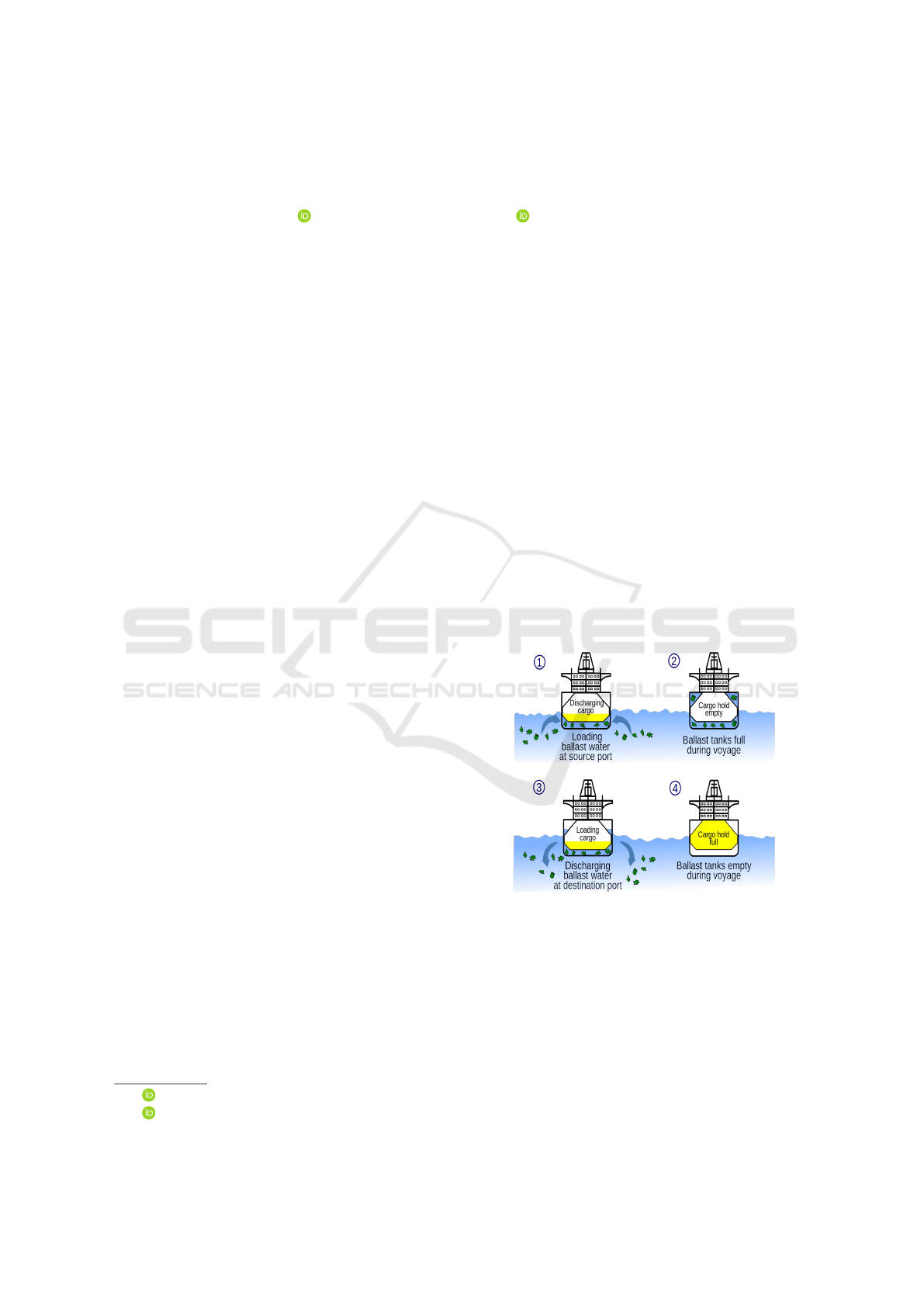
especially due to the discharge of ballast water. Bal-
last water is water that is taken on board by ships to
maintain their stability and balance (see Fig. 1). How-
ever, ballast water can also contain various microor-
ganisms, such as bacteria, viruses, algae and plank-
ton, that can be harmful to the ecosystems and human
health of the receiving regions.
A solution for ballast water treatment is an auto-
mated system that employs ultraviolet (UV) light and
filters to sanitize and cleanse the ballast water. This
system is governed by a programmable logic con-
troller (PLC) that oversees and modifies the opera-
tional parameters based on the water quality and flow
rate. However, optimizing this system’s performance
is a challenge due to various factors such as sensor
errors, system faults, water quality or environmen-
tal changes. Furthermore, the different standards and
regulations for ballast water quality in various regions
a
https://orcid.org/0000-0003-4872-8546
b
https://orcid.org/0000-0001-5133-6688
Figure 1: Ballasting and deballasting (wikipedia.org).
and countries can lead to logistical issues and delays
in fleet operations. Hence, there is a need for a so-
lution that can utilize sensor data and machine learn-
ing to enhance this system’s performance and prevent
failures or malfunctions.
The paper introduces an innovative approach that
leverages online machine learning to dynamically and
adaptively optimize the performance of ballast wa-
ter management systems (BWMS). Unlike traditional
methods relying on static or offline models, this novel
Iftikhar, N., Lin, Y., Liu, X. and Nordbjerg, F.
Online Machine Learning for Adaptive Ballast Water Management.
DOI: 10.5220/0012728700003756
Paper published under CC license (CC BY-NC-ND 4.0)
In Proceedings of the 13th International Conference on Data Science, Technology and Applications (DATA 2024), pages 27-38
ISBN: 978-989-758-707-8; ISSN: 2184-285X
Proceedings Copyright © 2024 by SCITEPRESS – Science and Technology Publications, Lda.
27

solution continuously trains and updates models us-
ing real-time sensor data from ships and ports. By
doing so, it gains insights into the complex and evolv-
ing patterns of ballast water quality, flow rate and the
diverse conditions encountered by ships and ports.
Additionally, the proposed solution provides prob-
abilistic forecasts, accounting for uncertainties in fu-
ture events that could impact BWMS performance
(Sayinli et al., 2022). Ultimately, the online machine
learning offers more precise and timely predictions,
effectively addressing the critical challenges associ-
ated with ballast water treatment in maritime transport
and environmental protection.
The main contributions of this paper are as fol-
lows:
• This paper proposes an online machine learn-
ing solution that accommodates various machine
learning models and algorithms tailored for dis-
tinct training objectives and strategies.
• This paper suggests three training strategies:
continuous training, scheduled training and
threshold-triggered training.
• The effectiveness and reliability of the presented
solution are demonstrated using real-world data
from ship and port performances. The results are
effectively visualized through various charts and
maps.
The rest of this paper is organized as follows: Sec-
tion 2 reviews related work. Section 3 defines the
problem. Section 4 introduces the online machine
learning approach that utilizes a variety of training
strategies. Section 5 describes the implementation de-
tails. Section 6 reports experimental results of the so-
lution. Section 7 summarizes the main contributions
and discusses future directions.
2 LITERATURE REVIEW
The effective management of ballast water using ad-
vanced analytical technologies is a topic of ongoing
research and development in the maritime industry
(Katsikas et al., 2023), with machine learning offering
the possibility to optimize the performance of BWMS
and mitigate their environmental impact. Predictive
maintenance is an important application of machine
learning in industrial systems. It aims to predict the
failure of machines or components before they occur
and to schedule maintenance activities accordingly.
This can improve the efficiency and reliability of in-
dustrial systems and reduce their downtime and main-
tenance costs (Kusiak and Li, 2011; Iftikhar et al.,
2022). Several machine learning techniques have
been proposed for predictive maintenance, including
supervised learning, unsupervised learning and rein-
forcement learning. Supervised learning techniques,
such as classification and regression, can be used to
predict the failure of machines or components based
on historical data (Chang and Lin, 2011; Hsu and
Lin, 2002; Japkowicz and Shah, 2011). Unsupervised
learning techniques, such as clustering and anomaly
detection, can be used to identify abnormal patterns
or behaviors in the data (Domingos and Hulten, 2000;
Iftikhar and Dohot, 2022). Reinforcement learning
techniques, such as Q-learning and actor-critic meth-
ods, can be used to optimize the maintenance policies
or schedules (Russell and Norvig, 2020).
Online machine learning is a sub-field of machine
learning that deals with data streams that arrive se-
quentially over time. Online machine learning algo-
rithms update their models incrementally as new data
arrives, without requiring access to the entire data
set at once. This makes them suitable for applica-
tions where the data is large, fast-changing, or non-
stationary. Online machine learning has been applied
to various domains, including computer vision, natu-
ral language processing, speech recognition and pre-
dictive maintenance (Bifet et al., 2023). In the context
of BWMS, online machine learning can be used to
optimize their performance by leveraging sensor data
from ships and ports. This can be formulated as a re-
gression problem or a classification problem depend-
ing on the desired performance indicators. Several
online machine learning algorithms can be used for
this purpose (Celik et al., 2023; Lyu et al., 2023; Bot-
tou, 2010; Chen and Guestrin, 2016).
Furthermore, training strategies for machine
learning models are important for achieving good per-
formance and generalization. Various training strate-
gies have been proposed in the literature (Wu et al.,
2020; Ling et al., 2016; Pedregosa et al., 2011; Hin-
ton et al., 2012; Duchi et al., 2011; Caruana et al.,
2004; Kim and Woo, 2022). These strategies aim to
improve model selection, parameter estimation, fea-
ture selection or error estimation of machine learn-
ing models. Similarly, model validation, which re-
lies on assessing a model’s performance and involves
retraining the model with new data, is a critical yet
demanding aspect of machine learning. These tasks
necessitate careful monitoring, efficient data manage-
ment and the application of sophisticated engineering
practices (Schelter et al., 2018). In addition, model
switching, as a concept in machine learning, is a dy-
namic and integrated operation. It is characterized
by continuous monitoring and anticipation of future
job arrivals and deadline constraints. The selection of
models and configurations is driven by data dynamics
DATA 2024 - 13th International Conference on Data Science, Technology and Applications
28

and the goal of achieving the highest effective accu-
racy. The system then implements the selected model
and configuration in real-time while serving predic-
tion requests. This process is further refined by the
incorporation of dynamic time warping for data seg-
mentation and proactive training for model updates.
Collectively, these strategies contribute to superior
model quality, thereby optimizing the overall perfor-
mance of the system (Zhang et al., 2020; Pinto and
Castle, 2022; Prapas et al., 2021).
Some of the weaknesses of previous work in this
field include not considering enough variability in
sensor data which could affect prediction accuracy;
not updating models frequently enough which could
lead to model drift; or not providing practical usabil-
ity which could limit validity or applicability in real-
world scenarios. This paper addresses these issues
by using probabilistic forecasting techniques that cap-
ture uncertainty; using online machine learning tech-
niques that update models incrementally; using vari-
ous training strategies; building a demonstrator to en-
sure desired functionality. The paper makes a signifi-
cant contribution to the field of BWMS.
3 PROBLEM FORMULATION
The management of ballast water is a critical issue in
maritime transport, as it can contain invasive species
and pathogens that pose a threat to the ecosystems and
human health of the receiving regions. Ensuring the
optimal performance of BWMS is challenging due to
various factors, including differences in water quality
and weather conditions at each port. To address this
challenge, a novel approach is proposed that utilizes
historical data on individual ship performance at each
port, as well as aggregate ship performance based on
flow rate. Flow rate represents the volume of ballast
water passing through a pipe’s cross-section within a
specific time frame. Additionally, the approach incor-
porates water quality and weather data for each port to
determine the optimal model for forecasting the flow
rate performance of a specific ship at a particular port.
Formally, let X
t
∈ R
d
denote the d-dimensional in-
put data at time t, which consists of sensor readings
from ships and ports, such as temperature, salinity,
turbidity, UV intensity, flow rate, etc., as well as wa-
ter quality and weather data at each port. Let Y
t
∈ R
denote the output data at time t, which consists of
the desired performance indicator of the BWMS. In
this paper, the flow rate is focused on as the main
performance indicator, as it reflects the efficiency
and effectiveness of the BWMS. The other perfor-
mance indicators could be disinfection rate, energy
consumption, etc. The goal is to find a sequence of
models m
1
,m
2
,...,m
t
that minimize the expected loss
E[L(Y
t
,
ˆ
Y
t
)], where
ˆ
Y
t
= M
t
(X
t
) is the predicted output
at time t and L : R × R → R is a loss function that
measures the discrepancy between the predicted out-
put and the actual output.
4 METHODS
4.1 Overview
The core concept of the suggested adaptive online ma-
chine learning technique involves utilizing a collec-
tion of potential machine learning models and choos-
ing the most effective one for predicting BWMS per-
formance indicators, drawing on sensor data from
ships and ports. Various training approaches are em-
ployed to update the models in response to different
circumstances.
Input: A stream of sensor data
X = {x
1
,x
2
,...,x
n
} from ships and
ports, a training strategy S
Output: A stream of predictions
ˆ
Y = { ˆy
1
, ˆy
2
,..., ˆy
n
} and their
confidence intervals
ˆ
C = { ˆc
1
, ˆc
2
,..., ˆc
n
}
Initialize a set of candidate machine learning
models M with random parameters θ;
Initialize a null best model m
∗
;
Initialize a null training trigger T ;
for i = 1 to n do
Receive a new input x
i
;
Predict the output ˆy
i
= m
∗
(x
i
;θ) and its
confidence interval ˆc
i
using the best
model;
Output ˆy
i
and ˆc
i
;
Update the training trigger T based on the
training strategy S;
if T is activated then
Train or update the models M using
the available data (X,Y );
Update the parameters θ;
Evaluate the models M using
performance metrics;
Select the best model m
∗
from M
based on the metrics and the
suitability for the ship-port pair;
end
end
Algorithm 1: Online Machine Learning.
The proposed method is capable of adapting to al-
Online Machine Learning for Adaptive Ballast Water Management
29

terations in data distribution and system dynamics and
can transition between different models depending on
their performance and appropriateness for the specific
ship-port combination. Algorithm 1 depicts the gen-
eral workflow of the proposed method, which is com-
prised of four steps: prediction, output, training trig-
ger and model selection. In the prediction step, the
best model from a set of candidate machine learning
models is used to predict the output and its confidence
interval for each new input data point. The confidence
interval signifies the uncertainty of the prediction and
can be utilized to gauge its reliability. In the output
step, the prediction and its confidence interval are re-
layed to the user. In the training trigger step, a trig-
ger is updated based on a predefined training strategy
that determines when to update the models. The trig-
ger can be activated by various criteria, such as data
availability, time intervals and/or error rates.
4.2 Model Training Strategies
The proposed method employs three training strate-
gies to update the models according to different con-
ditions: continuous training, scheduled training and
threshold-triggered training. These strategies differ in
how they activate the training trigger and how they
balance the trade-off between accuracy and efficiency.
4.2.1 Continuous Training
This strategy updates the models after each new in-
put data point, regardless of the performance or suit-
ability of the current model. It aims to capture the
most recent changes in the data distribution and sys-
tem dynamics. Formally, let M = {m
1
,m
2
,...,m
n
}
be a set of candidate machine learning models, D =
{D
1
,D
2
,...,D
t
} be a sequence of training data, where
D
t
represents the data available at time t, and let
P(m,D
t
) be a performance function that measures the
performance of model m on data D
t
. The continuous
training strategy is outlined in Algorithm 2.
The mathematical formulation of this strategy can
be expressed as follows:
m
(t+1)
current
= arg max
m∈M
P(m,D
t+1
)
where m
(t+1)
current
denotes the current model at time t + 1
and argmax denotes the argument that maximizes the
function.
This strategy is suitable for applications where
computational resources are abundant and where the
data distribution changes rapidly over time. How-
ever, it can be computationally expensive and prone
to overfitting as it requires training or updating the
models after each new input data point.
Function ContinuousTraining(M , D, P)
Initialize the current model m
current
as an
arbitrary model from M
for each time step t do
Update m
current
with new data D
t
Evaluate the performance of all
models in M on data D
t
using
P(m,D
t
)
if there exists a model m ∈ M such
that P(m,D
t
) > P(m
current
,D
t
) then
Update the current model as
m
current
= m
end
end
return
Algorithm 2: Continuous Training.
4.2.2 Scheduled Training
This strategy updates the models at fixed time inter-
vals, regardless of the performance or suitability of
the current model. It aims to reduce the computa-
tional cost and latency of the solution. Formally, let T
be a fixed time interval and let the other notations be
the same as in the previous strategy. The continuous
training strategy is outlined in Algorithm 3.
Function ScheduledTraining(M , D, P,
T )
Initialize the current model m
current
as an
arbitrary model from M
for each time step t do
if t mod T == 0 then
Update m
current
with new data D
t
Evaluate the performance of all
models in M on data D
t
using
P(m,D
t
)
if there exists a model m ∈ M
such that
P(m,D
t
) > P(m
current
,D
t
) then
Update the current model as
m
current
= m
end
end
end
return
Algorithm 3: Scheduled Training.
The mathematical formulation of this strategy can
be expressed as follows:
m
(t+T )
current
= arg max
m∈M
P(m,D
t+T
)
where m
(t+T )
current
denotes the current model at time t + T
DATA 2024 - 13th International Conference on Data Science, Technology and Applications
30

and argmax denotes the argument that maximizes the
function.
This strategy is more computationally economical
compared to continuous training as it requires train-
ing or updating the models only at fixed time inter-
vals. However, it might be slower in adapting to
rapid changes in data distribution or switching models
when performance drops.
4.2.3 Threshold-Triggered Training
This strategy updates the models when a certain
threshold is reached. It aims to maintain optimal per-
formance by monitoring and refining the models. For-
mally, let ε be a fixed threshold, let e be an error rate
calculated by comparing the predicted output with the
actual output and let the other notations be the same
as in the previous strategies. The threshold-triggered
training strategy is outlined in Algorithm 4.
Function
ThresholdTriggeredTraining(M , D, P,
ε)
Initialize the current model m
current
as an
arbitrary model from M
Initialize the error rate e as zero
for each time step t do
Update m
current
with new data D
t
Calculate the error rate e by
comparing the predicted output with
the actual output
if e ≥ ε then
Train or update all models in M
using new data D
t
Evaluate the performance of all
models in M on data D
t
using
P(m,D
t
)
if there exists a model m ∈ M
such that
P(m,D
t
) > P(m
current
,D
t
) then
Update the current model as
m
current
= m
end
Reset the error rate e as zero
end
end
return
Algorithm 4: Threshold-Triggered Training.
The mathematical formulation of this strategy can
be expressed as follows:
m
(t+1)
current
=
(
m
(t)
current
, if e < ε,
argmax
m∈M
P(m,D
t+1
), if e ≥ ε.
where m
(t+1)
current
and m
(t)
current
denote the current model at
time t +1 and t, respectively. Further, argmax denotes
the argument that maximizes the function.
This strategy can be computationally efficient as
it only requires training or updating the models when
the error rate exceeds a fixed threshold. This method
ensures that the models maintain optimal perfor-
mance by addressing the need for constant monitoring
and refinement.
4.3 Model Switching
Model switching is a technique that allows the selec-
tion of the best model from a set of candidate mod-
els based on their performance and suitability for the
given data and task. Model switching can enhance the
accuracy and robustness of the solution by adapting to
changes in the data distribution and system dynamics.
In this context, model switching is used to forecast the
performance indicators of BWMS using sensor data
from ships and ports.
Function ModelSwitching(M, D
train
, D
val
,
P)
for each model m ∈ M do
Train model m on the training data
D
train
Evaluate the performance of model m
on the validation data D
val
using the
performance function P(m,D
val
)
end
Select the best model m
∗
∈ M according
to the chosen criteria, i.e.,
m
∗
= argmax
m∈M
P(m,D
val
)
return m
∗
as the current model
return
Algorithm 5: Model Switching with Performance Evalua-
tion.
Different machine learning models are trained and
evaluated on the data and the best one is selected ac-
cording to the chosen criteria. Formally, let M =
{m
1
,m
2
,...,m
n
} be the set of available machine learn-
ing models, D
train
be the training data, D
val
be the val-
idation data and P(m,D) be the performance of model
m ∈ M on data D according to the chosen criteria. The
model switching process is outlined in Algorithm 5.
The model switching technique enables the selection
of the most suitable model for forecasting the perfor-
mance indicators of BWMS for each ship-port pair.
The performance evaluation is based on mean squared
error (MSE) and root mean squared error (RMSE).
The model switching can be triggered by any of the
training strategies mentioned earlier.
Online Machine Learning for Adaptive Ballast Water Management
31

5 IMPLEMENTATION
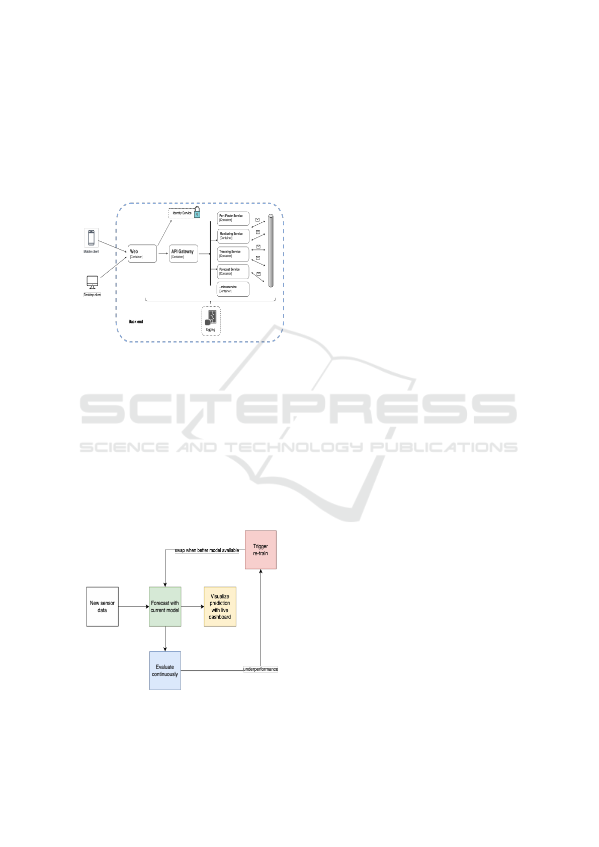
5.1 Architecture Overview
The online machine learning solution architecture
consists of four main components: a web front-end,
an identity service, an API gateway and a set of micro-
services (see Fig. 2).
Figure 2: Robust service architecture for online machine
learning.
The web front-end provides a user interface for ac-
cessing the system and visualizing the data and fore-
casts. The identity service handles authentication and
authorization of users and services. The API gateway
acts as a single entry point for all requests from the
web front-end to the back-end services. It also pro-
vides load balancing, routing, security and logging
functions. The set of micro-services implement the
online machine learning architecture, which is based
on an online machine learning workflow that continu-
ously trains and updates models based on sensor data
from ships and ports.
Figure 3: Online machine learning workflow: threshold-
triggered strategy.
The online machine learning solution architecture
consists of various microservices, some of the in-
teresting ones are: training service, forecast service,
model service and monitoring service. Training ser-
vice trains machine learning models based on differ-
ent training targets (such as, ships or ports) and strate-
gies. Forecast service generates forecasts using the
current models and save them to the database. Model
services implement different machine learning algo-
rithms for forecasting. Monitoring service evaluates
the performance of the models and triggers re-training
when needed. Considering the efficiency and com-
plexity of online machine learning architecture, inter-
nal services communicate using asynchronous mes-
saging. One important feature of this architecture is
its ability to switch between different models based on
their performance. This is achieved through a model
selection process (see Fig. 3) that compares the per-
formance of different models using various evaluation
metrics. The best performing model is then selected
and used for generating forecasts until a new selection
process is triggered.
5.2 Technologies
The implementation overview of the online machine
learning solution demonstrates its deployment and in-
tegration with other systems and technologies (see
Fig. 4). The solution is hosted on Azure Kubernetes
Service, which manages containerized applications
and provides scalability, reliability and security fea-
tures. Additionally, Azure IoT Hub is utilized to re-
ceive sensor data from devices on ships, while Azure
Functions process this data and send it to RabbitMQ.
The RabbitMQ data is then routed to microservices
and stored in TimescaleDB—a robust database cho-
sen for its excellent time-series data analysis capabil-
ities. For instance, to perform time-series forecasting,
the data is automatically aggregated into one-minute
intervals using a materialized view.
The system includes services related to training
strategies (such as the port and ship scheduler and
monitoring service) and machine learning (including
forecast, training and model services). Fitted ma-
chine learning models are stored separately in a Post-
greSQL database, which contains essential informa-
tion such as the model’s target, type/name, times-
tamp, fitted model checkpoint and the model itself.
Finally, Grafana dashboards visualize predictions and
live sensor data, enabling end-users to monitor system
performance. The online machine learning architec-
ture employs an asynchronous messaging system to
facilitate communication among microservices. This
messaging system comprises a message broker and a
DATA 2024 - 13th International Conference on Data Science, Technology and Applications
32

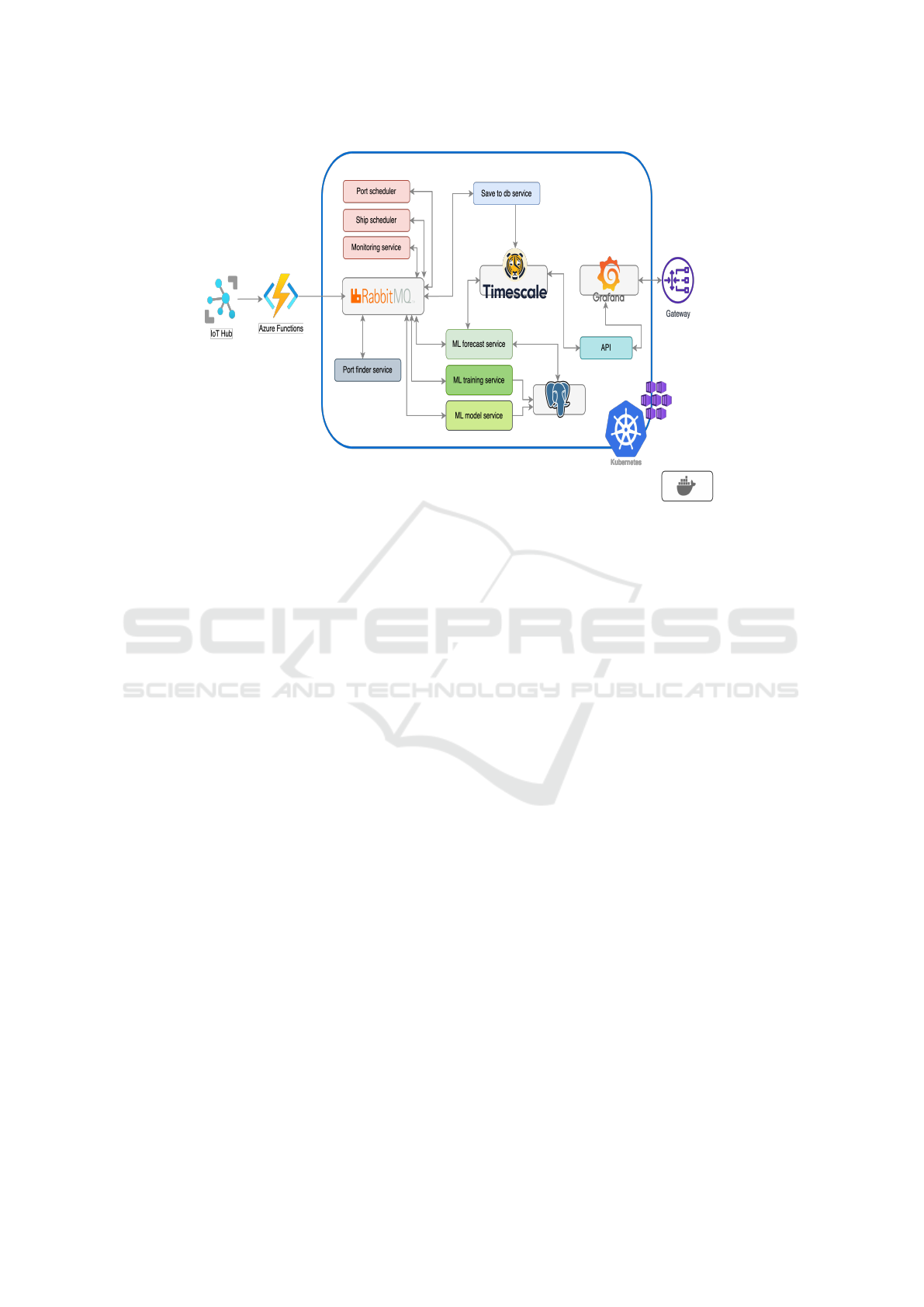
Figure 4: Service-oriented architecture with modern technologies: a robust and scalable approach.
collection of channels. Further details about this mes-
saging system are provided in the subsequent subsec-
tions.
5.3 Application in Ballast Water
Management Systems
This section explores how machine learning work-
flows are applied within the context of enhancing
BWMS. It centers around two primary tasks: Model-
ing and Forecasting. These tasks provide insights into
the practical application and efficient management of
machine learning techniques.
5.3.1 Modeling Task
The Modeling task outlines how the architecture de-
sign integrates into the machine learning workflow
(see Fig. 5 (a)). This task involves training machine
learning models for various ports and ships using
combined and preprocessed sensor data. The archi-
tecture comprises a sender, a message filter and two
types of training services (one for ports and one for
ships). The sender dispatches training requests with
a mixed message containing the training target and
a command. The message filter routes messages to
the appropriate point-to-point channels based on the
command. Subsequently, the training services extract
messages from the channels and train models using
data from the database. These trained models are then
stored in the database in binary format. The use of a
publish-subscribe channel and the message filter pat-
tern enhances design flexibility and scalability, allow-
ing for seamless participant additions or removals
5.3.2 Forecasting Task
The Forecasting task provides a detailed look into
the architecture design incorporated into the machine
learning workflow for generating forecasts (see Fig. 5
(b)). This task involves several components: The
sender dispatches forecast requests with a combined
message containing the target, the number of predic-
tions and the table name. The message filter routes
messages to the appropriate point-to-point channels
based on the model name. Subsequently, machine
learning model services (such as Recurrent Neural
Network (RNN) or Temporal Convolutional Network
TCN) consume messages from these channels and
generate forecasts using models from the database.
These forecasts are then stored in the database within
the specified table.
In this setup, forecast services receive messages
from a channel and retrieve the latest machine learn-
ing model name as a command. For example, if the
best model for Ship A is an RNN, the command mes-
sage would be Model:RNN. The Message Filter then
directs messages to the relevant channels based on the
command. Different machine learning model services
consume these messages. This design enables seam-
less integration of multiple machine-learning models
from various providers without altering the code in
the services.
Online Machine Learning for Adaptive Ballast Water Management
33

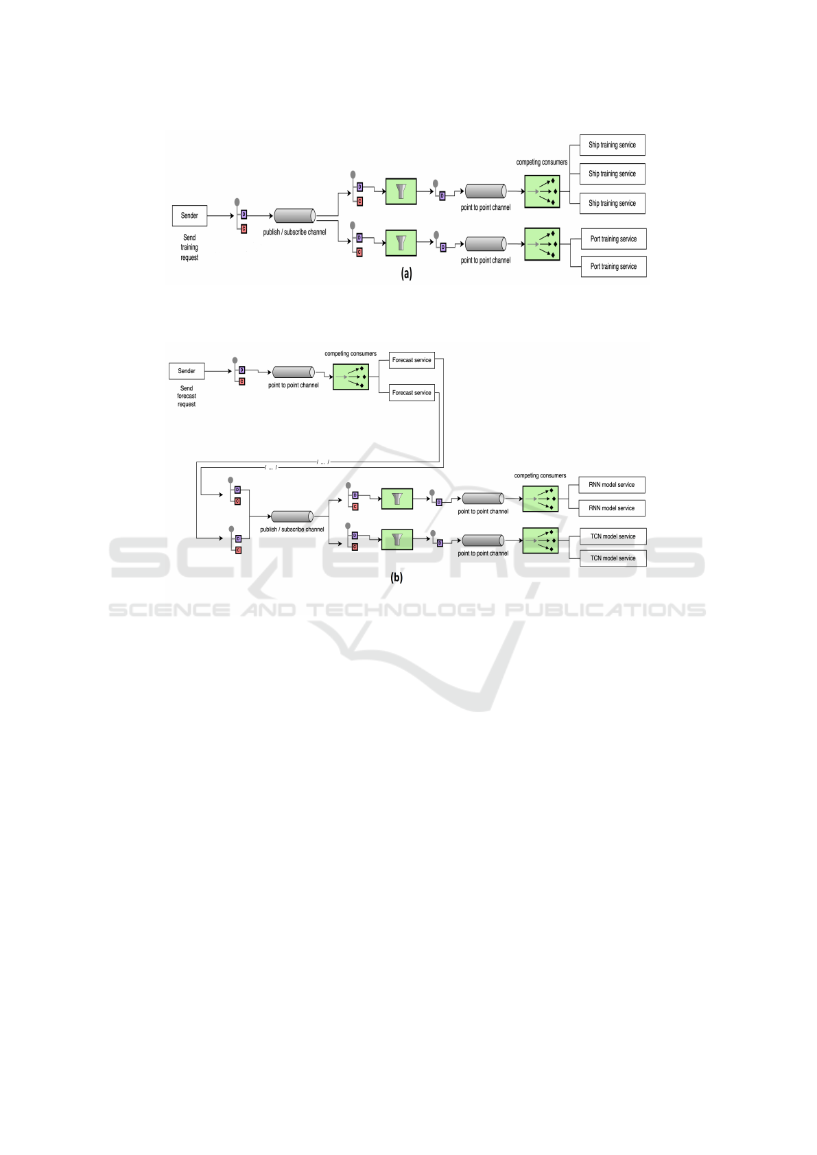
Figure 5: (a) Architecture diagram of modeling task; (b) Architecture diagram of forecasting task.
6 EXPERIMENTS
6.1 Data and Scenarios
To evaluate the solution, real sensor data from ships
and ports is utilized. This data encompasses measure-
ments such as temperature, salinity, turbidity, UV in-
tensity and flow rate. Along with information about
water quality and weather conditions at each port.
Real scenarios reflecting the operational conditions
of ships and ports are also employed in the experi-
ments. Although the data source remains undisclosed
to safeguard the privacy of the concerned individuals
or organizations, some general information about the
data, such as its size, distribution and characteristics,
is provided without revealing its origin.
The data sets offer a comprehensive insight into
port performances, ship ballast water management
readings and a detailed listing of ports. Performance
metrics for 473 ports spread across 65 countries. Ad-
ditionally, the data encompasses half a million entries
from 23 ships spanning from October, 2022, to June,
2023.
The analysis of maritime data, especially when fo-
cused on BWMS, presents multifaceted challenges.
BWMS, generate intricate data patterns influenced by
ship operations and the varying conditions at differ-
ent ports. Each ship, with its unique operational at-
tributes and BWMS configurations, interacts distinc-
tively with the diverse environmental and logistical
conditions inherent to individual ports. Ports them-
selves, with their fluctuating operational parameters,
can yield differing BWMS performance metrics for a
given ship. Moreover, external factors, potentially not
encapsulated within the data set, can exert significant
influence on BWMS performance and effectiveness.
The interplay of ships, ports and ballast management
underscores the need for comprehensive data prepro-
cessing, sophisticated modeling techniques and rig-
orous validation to derive meaningful and actionable
insights from the data set.
DATA 2024 - 13th International Conference on Data Science, Technology and Applications
34

6.2 Evaluation Methodology
A loss function L and a performance metric P with
cross-validation are used to evaluate and compare dif-
ferent machine learning models. Performance met-
rics evaluate the quality of predictions during test-
ing, while loss functions gauge the model’s perfor-
mance during training. The Mean Squared Error
(MSE) serves as the chosen loss function L. For time-
series data in cross-validation, the rolling RMSE is
employed as the performance metric P because of its
clear interpretability and resilience to outliers. Both
these metrics are widely recognized and have demon-
strated their effectiveness in numerous time series ap-
plications. Furthermore, cross-validation splits the
data into k folds, trains the model on k − 1 folds and
tests it on the remaining fold. This process is repeated
k times and the average performance serves as an es-
timate of the model’s generalization performance.
6.3 Models Presentation
A list of models M is introduced that encompasses
various machine learning models suitable for time-
series forecasting. These models can function as
probabilistic models, employing diverse algorithms
and architectures to generate predictions. Probabilis-
tic forecasting assigns a probability distribution to po-
tential outcomes of a future event, rather than just
predicting a singular value. For instance, instead of
forecasting that the ship flow rate will be 750 m
3
/h,
a probabilistic forecast might indicate a 50% proba-
bility that the flow rate will range between 650 and
850m
3
/h, a 25% likelihood of it being less than
650m
3
/h, and a 25% chance of exceeding 850m
3
/h.
The models in M include Temporal Convolutional
Network (TCN), Recurrent Neural Network (RNN),
Temporal Fusion Transformer (TFT) and Transformer
(T). TCN is a deep neural network that uses causal
convolution layers to capture long-term dependen-
cies in sequential data. TCN has the advantages
of parallelism, stable gradients and low memory re-
quirements. RNN is another deep neural network
that uses recurrent units to process sequential data.
RNN can learn from variable-length inputs and out-
puts, but it suffers from vanishing or exploding gra-
dients and high computational costs. TFT is a hybrid
model that combines convolutional, recurrent and at-
tention mechanisms to fuse temporal data from multi-
ple sources. TFT can handle complex and noisy data,
but it requires careful design and tuning of its compo-
nents. T is a deep neural network that relies solely on
attention mechanisms to encode and decode sequen-
tial data. T can learn long-range dependencies and
parallelize computations, but it needs large amounts
of data and regularization techniques to avoid over-
fitting. Each model m ∈ M is trained on the scaled
training data D
train
and subsequently used to predict
the validation data D
val
. The loss function L computes
the MSE of each model’s prediction ˆy and returns it
alongside the model, prediction and score. After ev-
ery training or re-training cycle for all models asso-
ciated with a ship or port, the top-performing model,
accompanied by a timestamp, is stored in the database
for subsequent retrieval. This mechanism ensures that
the most up-to-date model linked to a particular ship
or port can be retrieved, using the latest timestamp
during forecasting.
6.4 Dashboard and Result Analysis
The forthcoming visualizations provide a graphical
representation of the dashboard. To safeguard the
confidentiality of the data, actual information pertain-
ing to ships and ports has been removed. Fig. 6 (a)
depicts the actual and predicted flow rate of one of
the vessels, utilizing line charts based on temporal
data. The blue data points correspond to the observed
flow rate at each moment, selectively displaying sen-
sor data during active ballast operations. The orange
line represents the median (50%) of the probabilis-
tic forecast generated by the machine learning models
employed in this study. The light blue-shaded region
delineates the probabilistic forecast range spanning
from 5% to 95%, signifying the inherent uncertainty
in the prediction. Fig. 6 (a) reveals that the real-time
flow rate and the forecasted flow rate generally exhibit
alignment, although sometimes they differ. Notably,
there are instances where the ship’s live flow rate
surpasses the forecasted flow rate, indicating perfor-
mance that exceeds expectations. Conversely, around
15:00 on June 9th, the live flow rate marginally falls
below the forecasted flow rate, suggesting suboptimal
performance during that period. Additionally, the fig-
ure illustrates temporal fluctuations in the flow rate,
reaching a peak of approximately 97% around 13:00
on June 6th and dipping to approximately 85% around
14:30 on the same day. These observations provide
insights into the ship’s operational performance and
the model’s accuracy over time.
Additionally, Fig. 6 (b) presents a graphical dis-
play of the real-time and predicted flow rate for one
of the ports, represented through chronological line
charts. Each dot symbolizes a ship’s performance at a
specific instant, revealing only the sensor data during
the ballast operation. Different colors are used to dif-
ferentiate between ships. The actual value of the flow
rate is not displayed due to the existence of various
Online Machine Learning for Adaptive Ballast Water Management
35

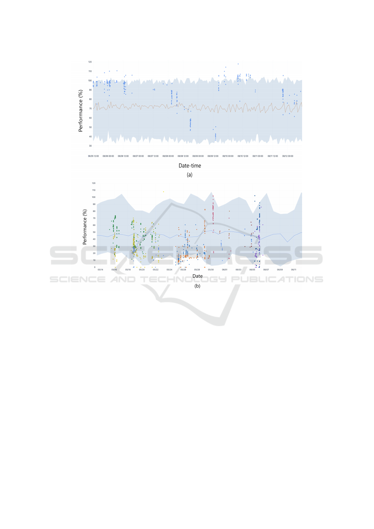
Figure 6: (a) One of the ship’s live and forecast data visualized with time-based line charts; (b) One of the port’s live and
forecast data visualized with time-based line charts.
sizes of ballast water systems. For ships with smaller
systems, the flow rate may not match that of ships
with larger systems. Consequently, the flow rate is
transformed into a performance percentage for a con-
sistent comparison across ships. The performance of
the BWMS is determined by dividing the actual flow
rate by the system’s maximum treatment-rated capac-
ity (TRC). The TRC represents the highest flow rate
that the BWMS can effectively treat, depending on
water quality, system size, and system health condi-
tion. The performance is expressed as a percentage,
with a higher value indicating superior performance.
This performance metric allows for a standardized
comparison of different ships/ports. The port forecast,
similar to the ship forecast, is probabilistic. The blue
solid line represents the median (50%) of the predic-
tion, while the light blue area encompasses the prob-
abilistic forecasting result.
Moreover, Fig. 7 (a) provides an insightful analy-
sis of ship performances at a specific port using both
bar and line charts. The bar chart illustrates the av-
erage performance of individual ships, quantified as
a percentage of the maximum TRC of the BWMS.
Ships are color-coded for differentiation. For exam-
ple, the mean performance of Ship ID S45-J67 at this
particular port is 51.6%, which closely aligns with
the mean performance of all ships at this port. How-
ever, other ships at this port under-perform during the
selected time range. Simultaneously, the line chart
tracks performance over time. The solid blue line
depicts the median prediction, providing valuable in-
sights into future ship performance. Notably, it also
highlights the variability in performance trends across
different ships.
Similarly, Fig. 7 (b) extends its focus to port-level
performance, visualized on a map. Each point on the
map corresponds to a specific port, with the color in-
dicating the average ship performance at that loca-
DATA 2024 - 13th International Conference on Data Science, Technology and Applications
36

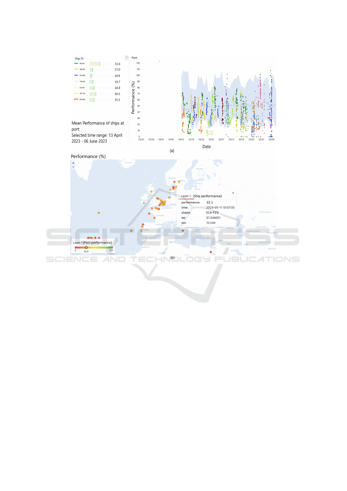
Figure 7: (a) Performance of ships at a specific port visualized with bar and time-based line charts; (b) Performance of each
port visualized with a map.
tion. The performance metric remains consistent, ex-
pressed as a percentage of the maximum TRC of the
BWMS. The color scale transitions from green (in-
dicating high performance) to red (indicating lower
performance). The interactive map enables users to
zoom in and hover over points for detailed informa-
tion. This geographical representation highlights the
performance variability across different regions and
countries, emphasizing the utility of maps in convey-
ing complex data relationships. In Fig. 7 (b), it is
observed that the mean performance of ships at this
specific port stands at 35.6%, with the selected ship
(S14-P23) falling slightly below the required perfor-
mance.
7 CONCLUSIONS AND FUTURE
DIRECTIONS
The paper introduces an innovative solution that uses
online machine learning to improve the efficiency of
ballast water management systems. The proposed ap-
proach is based on an online machine learning ar-
chitecture that can adapt to various machine learn-
ing models and algorithms, each tailored for specific
training goals and strategies. Three distinct training
strategies are described: continuous training, sched-
uled training and threshold-triggered training. By
utilizing real-world data from ship and port perfor-
mances, the solution’s effectiveness and reliability
are demonstrated. The results are visually presented
through various charts and maps.
In future research, the focus will be on enhanc-
ing the solution’s performance by forecasting over
a longer time horizon. This involves exploring ad-
Online Machine Learning for Adaptive Ballast Water Management
37

vanced machine learning models and algorithms, re-
fining training methods, augmenting sensor data from
ships and ports and addressing operational complexi-
ties specific to maritime environments. Additionally,
a comprehensive comparative analysis will assess the
pros and cons of online machine learning for adaptive
ballast water management.
REFERENCES
Bifet, A., Gavald
`
a, R., Holmes, G., and Pfahringer, B.
(2023). Machine Learning for Data Streams. The
MIT Press.
Bottou, L. (2010). Large-scale machine learning with
stochastic gradient descent. In Proceedings of the 19th
International Conference on Computational Statistics,
pages 177–186.
Caruana, R., Niculescu-Mizil, A., Crew, G., and Ksikes, A.
(2004). Ensemble selection from libraries of models.
In Proceedings of the 21st International Conference
on Machine Learning.
Celik, B., Singh, P., and Vanschoren, J. (2023). Online au-
toml: An adaptive automl framework for online learn-
ing. Machine Learning, 112(6):1897–1921.
Chang, C. C. and Lin, C. J. (2011). Libsvm: A library for
support vector machines. ACM Transactions on Intel-
ligent Systems and Technology, 2(3):1–27.
Chen, T. and Guestrin, C. (2016). Xgboost: A scalable
tree boosting system. In Proceedings of the 22nd
ACM SIGKDD International Conference on Knowl-
edge Discovery and Data Mining, pages 785–794.
Domingos, P. and Hulten, G. (2000). Mining high-speed
data streams. In Proceedings of the 6th ACM SIGKDD
International Conference on Knowledge Discovery
and Data Mining, pages 71–80.
Duchi, J., Hasan, E., and Singer, Y. (2011). Adaptive sub-
gradient methods for online learning and stochastic
optimization. Journal of Machine Learning Research,
12:2121–2159.
Hinton, G., Deng, L., Yu, D., Dahl, G., r. Mohamed, A.,
Jaitly, N., Senior, A., Vanhoucke, V., Nguyen, P.,
Sainath, T., and Kingsbury, B. (2012). Deep neural
networks for acoustic modeling in speech recognition.
IEEE Signal Processing Magazine, 29(6):82–97.
Hsu, C. W. and Lin, C. J. (2002). A comparison of methods
for multiclass support vector machines. IEEE Trans-
actions on Neural Networks, 13(2):415–425.
Iftikhar, N. and Dohot, A. M. (2022). Condition based
maintenance on data streams in industry 4.0. In Pro-
ceedings of the 3rd International Conference on Inno-
vative Intelligent Industrial Production and Logistics,
pages 173–144.
Iftikhar, N., Lin, Y. C., and Nordbjerg, F. E. (2022). Ma-
chine learning based predictive maintenance in manu-
facturing industry. In Proceedings of the 3rd Interna-
tional Conference on Innovative Intelligent Industrial
Production and Logistics, pages 85–93.
Japkowicz, N. and Shah, M. (2011). Evaluating Learning
Algorithms: A Classification Perspective. Cambridge
University Press.
Katsikas, S., Manditsios, G. N., Dalmiras, F. N., Sakalis, G.,
Antonopoulos, G., Doulgeridis, A., and Mouzakis, D.
(2023). Challenges to taking advantage of high fre-
quency data analytics to address environmental chal-
lenges in maritime sector. In Proceedings of the 8th
International Symposium on Ship Operations, Man-
agement and Economics.
Kim, J. and Woo, S. S. (2022). Efficient two-stage model
retraining for machine unlearning. In Proceedings of
the IEEE/CVF Conference on Computer Vision and
Pattern Recognition Workshops, pages 4361–4369.
Kusiak, A. and Li, W. (2011). The prediction and diagnosis
of wind turbine faults. Renewable Energy, 36(1):16–
23.
Ling, J., Jones, R., and Templeton, J. (2016). Machine
learning strategies for systems with invariance prop-
erties. Journal of Computational Physics, 318:22–35.
Lyu, Z., Ororbia, A., and Desell, T. (2023). Online evo-
lutionary neural architecture search for multivariate
non-stationary time series forecasting. Applied Soft
Computing, page 110522.
Pedregosa, F., Varoquaux, G., Gramfort, A., Michel, V.,
Thirion, B., Grisel, O., Blondel, M., Prettenhofer, P.,
Weiss, R., Dubourf, V., Vanderplas, J., Passos, A.,
Cournapeau, D., Brucher, M., Perrot, M., and Duch-
esnay, E. (2011). Scikit-learn: Machine learning
in python. Journal of Machine Learning Research,
12:2825–2830.
Pinto, J. M. and Castle, J. L. (2022). Machine learning dy-
namic switching approach to forecasting in the pres-
ence of structural breaks. Journal of Business Cycle
Research, 18(2):129–157.
Prapas, I., Derakhshan, B., Mahdiraji, A. R., and Markl, V.
(2021). Continuous training and deployment of deep
learning models. Datenbank-Spektrum, 21:203–212.
Russell, S. J. and Norvig, P. (2020). Artificial Intelligence:
A Modern Approach. Pearson, 4th edition.
Sayinli, B., Dong, Y., Park, Y., Bhatnagar, A., and Sil-
lanp
¨
a
¨
a, M. (2022). Recent progress and challenges
facing ballast water treatment–a review. Chemo-
sphere, 291:132776.
Schelter, S., Biessmann, F., Januschowski, T., Salinas, D.,
Seufert, S., and Szarvas, G. (2018). On challenges in
machine learning model management. Bulletin of the
IEEE Computer Society Technical Committee on Data
Engineering, 41(4):5–15.
Wu, Y., Dobriban, E., and Davidson, S. (2020). Deltagrad:
Rapid retraining of machine learning models. In Pro-
ceedings of the International Conference on Machine
Learning, pages 10355–10366.
Zhang, J., Elnikety, S., Zarar, S., Gupta, A., and Garg, S.
(2020). Model-switching: Dealing with fluctuating
workloads in machine-learning-as-a-service systems.
In Proceedings of the 12th USENIX Workshop on Hot
Topics in Cloud Computing.
DATA 2024 - 13th International Conference on Data Science, Technology and Applications
38