
Modelling Implicit and Explicit Communication Between Road
Users from a Non-Cooperative Game-Theoretic Perspective:
An Exploratory Study
Isam Bitar
a
, Albert Solernou Crusat
b
and David Watling
c
Institute for Transport Studies, University of Leeds, 34-40 University Rd, Leeds, LS2 9JT, U.K.
Keywords: Game Theory, Communication, Cheap Talk, Non-Cooperative Games, Bayesian Games,
Emergent Cooperation.
Abstract: Road user interaction is a fertile avenue for communication between road users, be it implicit communication
or explicit signals sent with the intent to convey information. To date, most literature on characterising and
modelling communication between road users has focussed on cooperative paradigms and concepts of shared
goals enforced globally on communicating agents. In this paper, we argue that non-cooperative game theory
can be used to characterise and model effective and mutually beneficial communication between road users.
We demonstrate that non-cooperative game theory can produce meaningful improvements in payoffs and
interaction safety for both the sender and recipient of communication as an emergent phenomenon.
1 INTRODUCTION
The reciprocal interaction between road users is a
fundamental part of the transport experience. The
modelling of such interaction is a rapidly growing
field. Game-theoretic models are one paradigm in
which interaction is studied (Ali et al., 2019; Elvik,
2014; Ji & Levinson, 2020; Kita, 1999), especially
from an autonomous vehicle’s perspective (Bitar et
al., 2022, 2023; Camara et al., 2019). Yet, few such
models pay attention to communication as a
participatory component of road user interaction. In
fact, recent work on road user communication as an
active component of interaction rejects the game-
theoretic approach in part due to its perception as a
framework that does not lend itself to communicative
behaviour (Siebinga et al., 2023). Instead, the
researchers rely on an underlying assumption of the
existence of a shared goal between interacting
players. Yet, non-cooperative game theory has been
extensively used to describe and explain emergent
cooperative and communicative behaviour in nature,
economics, society, and networking (Axelrod &
Hamilton, 1981; Fernández Domingos et al., 2017;
a
https://orcid.org/0000-0002-5130-0148
b
https://orcid.org/0000-0003-4857-0240
c
https://orcid.org/0000-0002-6193-9121
Orzan et al., 2023; Rubenstein & Kealey, 2010;
Stewart & Plotkin, 2013). In this paper, we argue that
non-cooperative game theory is a suitable framework
for modelling and describing communicative
behaviour between road users. We also argue that it
can produce beneficial cooperative behaviour as an
emergent property which does not require
assumptions of common goals or shared values.
We test three hypotheses in this study: 1) vehicles
have a selfish incentive to send communication
(explicit); 2) vehicles have a selfish incentive to
respond to communication (implicit and explicit); and
3) non-cooperative game theory can produce
meaningful, cooperative communication as an
emergent phenomenon which brings population-wide
benefits, quantified by: (a) average population payoff;
(b) number of crashes; and (c) number of near misses
(defined as interactions with
).
456
Bitar, I., Crusat, A. and Watling, D.
Modelling Implicit and Explicit Communication Between Road Users from a Non-Cooperative Game-Theoretic Perspective: An Exploratory Study.
DOI: 10.5220/0012729000003702
Paper published under CC license (CC BY-NC-ND 4.0)
In Proceedings of the 10th International Conference on Vehicle Technology and Intelligent Transport Systems (VEHITS 2024), pages 456-464
ISBN: 978-989-758-703-0; ISSN: 2184-495X
Proceedings Copyright © 2024 by SCITEPRESS – Science and Technology Publications, Lda.
2 METHOD
2.1 The Interaction Model
We conceptualise interactions as part of a lane-
change scenario. The interaction is a two-player,
sequential, non-cooperative game in which the Main-
lane Vehicle moves first, followed by a response
from the Joining Vehicle . The game is one of
imperfect information (Harsanyi, 1968). We
introduce two Bayesian elements and provide a
pathway to update beliefs based on communication:
and . (values:
/) relates to whether Vehicle
is aware of and responsive to Vehicle ’s movement.
(values: /) relates
to whether Vehicle is willing to accept a lane-
change if it is not in its favour. Both properties are
determined by with a pre-defined probability
for and for . has prior
knowledge of its own and will use this
knowledge in its decision-making. It does not have
knowledge of its own , and therefore this
attribute does not factor into the decision. If Vehicle
is , it has a further chance to be
and not take any action.
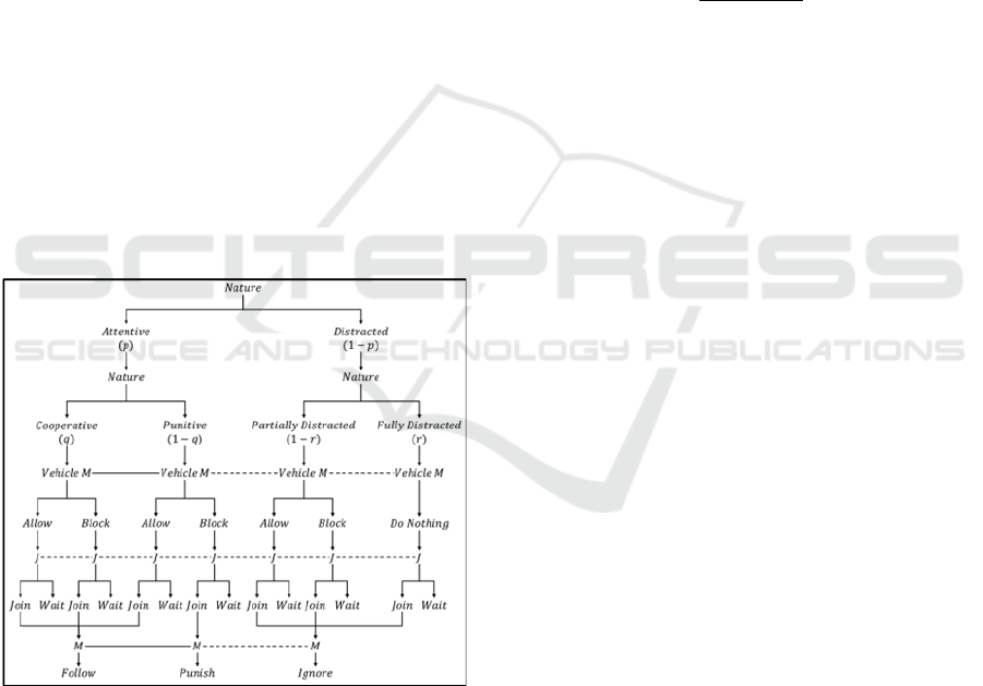
Figure 1: The extensive form sequential game between the
Main-lane Vehicle and the Joining Vehicle (game
tree).
The game continues as shown in Figure 1. A
action means Vehicle keeps a suitable
time headway. A action means tailgates
to induce a negative utility. An action means
continues moving as if it were in free flow and
does not take measures to prevent a collision. The
distraction state only lasts a finite amount of time,
after which Vehicle employs the equivalent
action (i.e. or ).
2.2 The Kinematic Model
Each vehicle possesses a set of attributes and
preferences unique to it. We explore the ranges used
for these properties in this study in the Experimental
Design section. The general movement of the two
vehicles is governed by a modified version of the bi-
directional General Motors (GM) Car Following
Model (Jin et al., 2013), which calculates the
acceleration of the following vehicle at timestep
as follows:
(1)
where:
is the acceleration of the agent vehicle at
the end of the next timestep .
is the velocity of the agent vehicle at the
current timestep .
is the distance difference between the agent
vehicle and its car-following target at timestep .
is the velocity difference between the agent
vehicle and its car-following target at timestep .
is a sensitivity factor which governs the agent
vehicle ’s corrective acceleration rate to maintain
car-following headway. The higher the sensitivity
factor, the more aggressive the correction.
are parametric sensitivity factors which in
this study are set to 1.
is constrained by the agent vehicle’s
acceleration preferences and physical limitations.
These are explored and described in Table 1.
The interaction begins at Timestep
= 0 when
Vehicle takes its first action.
’s duration is equal
to Vehicle ’s Decision Time
. The second timestep
begins once Vehicle takes its action and lasts an
amount of time equal to Vehicle ’s Decision Time
or after a certain period passes and may
assume has decided to . The third timestep
begins when Vehicle takes its second action. The
timesteps
and
are event-based, meaning their
durations are tied to the specific values of
and
in each interaction, respectively.
Vehicle will accelerate with the appropriate
if it wishes to Vehicle ’s attempt to .
This movement is not governed by the GM model.
Instead, will apply the appropriate
so that it
Modelling Implicit and Explicit Communication Between Road Users from a Non-Cooperative Game-Theoretic Perspective: An
Exploratory Study
457

would force a collision with within the lane change
manoeuvre duration
as follows:
(2)
where:
is the lane change duration.
is Vehicle ’s maximum acceleration.
is constrained as follows:
Vehicle will yield with the appropriate
if
it wishes to Vehicle to join ahead by
following it. The value of
is derived from Eq. 1
as shown in Table 1 (Eq. 3). Vehicle will maintain
until it observes an action from Vehicle or a
period of time passes after which assumes Vehicle
has decided to .
At the next timestep, if Vehicle decides to ,
it employs the appropriate
. This value is governed
by the formulae derived from Eq. 1 as shown in Table
1 (Eq. 4). Eq. 4(a) uses the car-leading element of the
bi-directional GM model where a leading vehicle
adjusts its velocity in response to the velocity of a
following vehicle. If Vehicle decides to , it
continues along its path at a constant speed until
passes (Eq. 5).
The remainder of the interaction is governed in
accordance with the general formula in Eq. 1 and
subject to the parameters and constraints shown in
Table 1 (Equations 1 through 7). The interaction
continues until a crash is detected or all the following
conditions are met:
▪
▪
▪
The equations of linear motion are used to
determine the values of the velocities and distances of
each vehicle at every timestep.
Table 1: General Motors car following model parameters and constraints as applied to Eq. 1.
Eq.
№
Action
Parameters
Special Cases
Constraints
3
or
4
(a)
:
(b)
:
-
:
:
5
-
-
6
7
where:
is the maximum possible deceleration to mitigate collision.
(Eq. 3) is used to ensure that the car following model does not push beyond its initial velocity
even if has a higher velocity
than
.
(Eq. 4) ensures accelerates to meet its
even if ’s velocity is lower than
.
The
employed in free flow (Eq. 4 and Eq. 7) is equal to the space covered in
seconds at the agent vehicle’s current
velocity (
or
). This creates a “phantom vehicle” which drives
seconds ahead for the agent vehicle to follow.
This is designed to give a gentle acceleration profile in free-flow situations.
VEHITS 2024 - 10th International Conference on Vehicle Technology and Intelligent Transport Systems
458

2.3 Communication
Communication in this model is issued by Vehicle
and received by Vehicle . We employ two forms of
communication: implicit communication,
characterised as the presence and value of
acceleration, and explicit communication, which is
either absent or present. When present, explicit
communication can be either positive or negative.
2.4 The Bayesian Elements
Vehicle is assigned two stochastic properties upon
its creation: () and
( ). Research
suggests that 1% of all drivers in the UK were
observed using a mobile phone in 2021 (DfT, 2022).
In this model, more exaggerated probabilities have
been chosen to amplify the effect for easier
observation. These base probabilities are known to
Vehicle as prior beliefs, therefore we do not expect
the general conclusions of this study to be affected by
the base values assigned to these probabilities. We
confine the purpose of communication to advertise
the two stochastic properties of Vehicle discussed
earlier. Vehicle will use these signals to update its
beliefs on Vehicle ’s stochastic properties in
accordance with Bayes’ Theorem (Joyce, 2021).
2.5 The Payoff Functions
Ride Comfort
We base ride comfort on both the acceleration values
at each timestep (with respect to the comfortable
value
) and the fluctuation of acceleration across
timesteps (best measured as the standard deviation of
acceleration about its mean). It is calculated is as:
(8)
where
is used in the denominator of the first term if
, else
.
is the total count of the interaction’s timesteps.
is the duration of timestep .
Time Headway
is a function of the minimum time headway
achieved during the interaction with respect to the
minimum acceptable headway
.
(9)
Speed difference
For Vehicle ,
is based on the difference between
the vehicle’s initial and final (steady state) velocities.
For Vehicle ,
is the difference between ’s
desired velocity and ’s final velocity if opts to
,. If chooses to ,
is a function of ’s
highest achieved velocity.
(10)
(11)
Time penalty
Vehicle is subject to
if it chooses to .
is
a function of the time needs to wait for to pass
before it can behind it. It is calculated as:
(12)
where
is a reduction factor used to normalise
with
respect to the other payoff components.
*
is used in this instance to prevent from
waiting indefinitely for a slower to pass
Table 2 summarises the payoff calculations based
on the action(s) taken.
Modelling Implicit and Explicit Communication Between Road Users from a Non-Cooperative Game-Theoretic Perspective: An
Exploratory Study
459

Table 2: Payoff summary per vehicle per action pair.
Action Pair
Vehicle
Vehicle
where
3 EXPERIMENTAL DESIGN
We run three simulation groups as follows:
Control Group. Vehicle does not engage in any
form of explicit communication. Vehicle relies
solely on the base probabilities of Vehicle ’s
and as prior beliefs. These
probabilities are outlined later in this section.
Test Group A. Vehicle does not issue any explicit
signals. Vehicle reads ’s acceleration as an
implicit signal to update its prior beliefs in line with
the likelihoods outlined in Table 6.
Test Group B. Vehicle employs explicit
communication signals as outlined in Table 5.
Each simulation group comprises a simulation of
30,000 interactions. Each interaction is a unique
iteration of Vehicle and Vehicle with attributes
and preferences which are randomly generated from
a uniform distribution of preset ranges. All three
simulation groups use the same random generator
seed. This allows for pairwise comparisons to be
made at the interaction level, including paired t-tests.
Table 3 outlines the different attributes and the
ranges from which they are generated. Table 4 lists
the constants defined in the Method section which are
used in all interactions and simulations in this study.
is assigned the property with a
probability . This property is concealed
from , i.e. it does not factor into ’s decision-
making. is assigned the property
with a probability . This property is known to
and factors into its decision-making. is assigned
the property with a probability
. This property is also concealed from .
Vehicle has prior knowledge of these base
probabilities, but no concrete knowledge of the
attribute assignment. It must assign a probability to
each of the three possible positions of Vehicle on
the game tree based on these prior beliefs.
Absent any other information, the probabilities
assigns to each of Vehicle ’s nodes (Figure 1) are:
▪ : 0.75×0.6 = 0.45
▪ : 0.75×0.4 = 0.3
▪ : 0.25
The state lasts for twelve timesteps
(5 - 8 seconds, based on the values of
and
)
after which Vehicle returns to its appropriate
actions as described in the Method section.
The entire experiment is conducted twice with
two different rulesets. In Ruleset 1 (Transparent),
both vehicles enjoy full knowledge of each other’s
properties (Table 3). Thus, both vehicles have
complete information, and the only element of
uncertainty comes from the Bayesian elements
described previously. In Ruleset 2 (Blind), both
vehicles are blind to each other’s properties and so
have incomplete information. They assume the
opponent has identical properties to their own where
applicable (otherwise a random value within the
ranges specified in Table 3 is used). Both vehicles
read each other’s velocities and positions accurately.
Table 3: Kinematic properties of the model and their ranges.
Property
Description
Value Range
Maximum comfortable acceleration
(0.20, 2.00) m/s
2
Maximum allowable acceleration
(2.50, 3.50) m/s
2
(Bokare & Maurya, 2017)
Maximum comfortable deceleration
(-0.50, -1.50) m/s
2
Minimum acceptable time headway
(0.50, 3.50) s
Decision time
(0.50, 1.50) s
Punitive sensitivity factor (exclusive to )
(0.15, 0.35)
Initial velocity
: (8.00, 18.00) m/s; : (4.00, 10.00) m/s
Initial distance (
as datum)
(5.00, 80.00) m
Desired velocity (exclusive to )
(0.75, 1.50) ×
m/s
penalty reduction factor
(0.10, 0.20)
VEHITS 2024 - 10th International Conference on Vehicle Technology and Intelligent Transport Systems
460

Table 4: list of constants used in the simulations and their values.
Constant
Description
Value
Lane change duration
5 seconds (Finnegan & Green, 1990; Salvucci & Liu, 2002)
GM model sensitivity factors
1
Timestep (from
onwards)*
0.5 seconds
Phantom vehicle time headway
4 seconds
Crash penalty
-250
Maximum safe deceleration
-4.5 m/s
2
(AASHTO, 2011; Bokare & Maurya, 2017)
* We set an upper limit of 60 time-based timesteps (
(30 seconds) for the duration of each interaction. The reason for
dictating this upper limit is computational efficiency for the computer model.
Table 5: Probabilities of Vehicle issuing various communicative signals.
Signal Category
Description
Probability of occurrence
Attentive
Distracted
Implicit: acceleration
alters its velocity as appropriate
1
0.5
Explicit: attention e.g. eye contact
makes eye contact with
0.9
0.05
Explicit: intention
e.g. gestures
issues a cooperative signal
Cooperative: 0.8; Punitive: 0.2
0.1
issues a threatening signal
Cooperative: 0.1; Punitive: 0.8
Table 6: Breakdown of the likelihoods of each signal given Vehicle 's different possible stochastic attributes.
Signal Category
Value
Description
Implicit: acceleration
0
observes no acceleration from
0.1*
0.1*
0.55
1
observes deceleration from
0.45*
0.3*
0.2
-1
observes acceleration from
0.45*
0.6*
0.25
Explicit: attention
e.g. eye contact
0
is unable to make eye contact with
0.1
0.1
0.95
1
makes eye contact with
0.9
0.9
0.05
Explicit: intention
e.g. gestures
0
does not observe an intention from
0.585*
0.415*
0.9
1
observes positive intent from
0.36*
0.09*
0.045
-1
observes negative intent from
0.055*
0.495*
0.055
* These
values are based on results obtained from a pilot simulation run of 10,000 interactions.
4 RESULTS
All three simulation groups were concluded
successfully. The results are aggregated, and key facts
presented in Table 7. The simulations produced
logical interaction behaviours. Vehicles behaved in a
predictable manner, favouring safer actions, and
avoiding unreasonable risks. The number of recorded
crashes and near misses was minimal (0.14% and
0.74% at maximum, respectively). The / -
/ split was balanced, with slight bias
towards / (average 44% and 53%,
respectively). This indicates a balanced distribution
of starting conditions and vehicle attributes. The
non-ideal outcomes (/ and /)
were minimal but non-trivial (average 1.6% and
1.1%, respectively).
We pay special attention to the occurrence of
non-ideal outcomes in this study, since such
outcomes indicate misinterpretation from one or both
road users in an interaction, and therefore would
prove a useful metric for gauging effective
communication between road users. Ruleset 1
produced fewer non-ideal outcomes across all three
groups than Ruleset 2. Similarly, Ruleset 1 proved the
safer of the two sets, with fewer near misses and
crashes than Ruleset 2. Ruleset 1 produced higher
average payoffs for both vehicles than Ruleset 2.
However, Ruleset 2 saw a higher percent increase for
both vehicles’ payoffs compared to Ruleset 1.
5 DISCUSSION
Non-ideal outcomes in the form of / and
/join are manifestations of one or more road
users misinterpreting an interaction. These outcomes
are considered non-ideal since Vehicle intends a
certain outcome, but Vehicle responds with a
different action. Such outcomes typically return
Modelling Implicit and Explicit Communication Between Road Users from a Non-Cooperative Game-Theoretic Perspective: An
Exploratory Study
461

worse payoffs to both vehicles than either of the ideal
alternatives (average -6.01 and -0.831, respectively).
In game theory, such outcomes are considered Pareto
inefficient. Pareto efficiency is a situation where no
player can receive a better payoff without causing
another to receive a worse payoff (Osborne, 2003).
Since either vehicle could have taken an alternative
action to improve at least its own payoff, such
outcomes are Pareto inefficient.
In Ruleset 1 (Transparent), the uncertainty around
Vehicle ’s and are the main
contributors to such outcomes. Since Vehicle has
knowledge of Vehicle ’s true attributes, the
acceleration value it employs to or
Vehicle is more likely to create an acceptable
environment for . This is why Ruleset 1 produces
fewer non-ideal outcomes over all compared to
Ruleset 2 (Blind). Furthermore, since Ruleset 1’s
interaction uncertainty is confined to only two
attributes, the effect of communication on Vehicle ’s
decision making is amplified. This is evident in the
total percent decrease in Ruleset 1’s non-ideal
outcomes which average 28.07%. Ruleset 2’s stands
at a more conservative 9.63%.
Similarly, Ruleset 1 produces fewer crashes (2
average) and near misses (38 average) than Ruleset 2
(12 and 70, respectively) as there is less room for
misinterpretation. In fact, outcomes
caused the bulk of crashes and near misses in all three
groups. It makes sense therefore that Ruleset 1 sees
fewer of these than Ruleset 2, all while enjoying a
greater percent decrease in both. Ruleset 1’s average
percent decrease in crashes and near misses from base
to full communication sits at 40.96%, whereas
Ruleset 2’s averages at only 9.13%. This is partly
because Ruleset 2 saw a rise in near misses in the test
groups over the control (17.46%). This suggests that
communication encouraged Vehicle to take more
risks. Interestingly, however, despite the increase in
near misses, there was a 35.71% reduction in crashes.
Active communication, it seems, has encouraged
Vehicle to take more risks, whilst also
refraining from taking potentially catastrophic risks.
Indeed, looking at average payoffs, we see further
evidence to corroborate this theory.
The average payoffs for both and are
predictably higher (better) in Ruleset 1 than Ruleset 2
(-0.668 vs -0.993). Having full knowledge of an
opponent’s attributes and preferences means both
vehicles can make accurate calculations on each
other’s movements and responses, resulting in fewer
over-all dangerous or undesirable interactions. Both
rulesets benefit from added communication. The
main difference is that Ruleset 1 saw the most benefit
going from no communication to implicit
communication, whereas Ruleset 2 saw the most
benefit going from implicit to full communication.
Since players under Ruleset 1 already play an
optimised game in which they have near-complete
information, implicit communication is sufficient to
provide Vehicle meaningful certainty on ’s
and . Further communication
(Group B) only serves to strengthen what is already
sufficiently known. On the other hand, when the
information available is either incomplete or
inaccurate, such as in Ruleset 2, explicit
communication becomes more vital as information
becomes more limited. Indeed, research shows that
Table 7: Summary of simulation results.
Metric
Ruleset 1 (Transparent)
Ruleset 2 (Blind)
None
(Control)
Implicit
(Group A)
Full
(Group B)
None
(Control)
Implicit
(Group A)
Full
(Group B)
Allow/Wait
162
166
119
191
193
166
Block/Go
81
64
57
167
153
156
Total near misses
47
35
32
63
74
74
Total crashes
2
1
1
14
12
9
Average payoff (Vehicle )
-0.776
-0.735
-0.731
-1.154
-1.085
-1.017
One-tailed paired t-test (vs Implicit)
-
< 0.01
0.31
-
0.02
< 0.01
One-tailed paired t-test (vs None)
-
-
< 0.01
-
-
< 0.01
Average payoff (Vehicle )
-0.619
-0.580
-0.569
-0.967
-0.909
-0.827
One-tailed paired t-test (vs Implicit)
-
< 0.01
0.11
-
0.04
< 0.01
One-tailed paired t-test (vs None)
-
-
< 0.01
-
-
< 0.01
VEHITS 2024 - 10th International Conference on Vehicle Technology and Intelligent Transport Systems
462

road users seek communication from others when
facing uncertainty (Portouli et al., 2014). Our results
corroborate these findings.
Finally, communication in both rulesets gave
statistically significant payoff improvements to both
Vehicle (the issuer) and Vehicle (the recipient).
Thus, cooperative communication can emerge from
selfish motives. These improvements were also
statistically significant with implicit communication
over control, meaning that active participation by
Vehicle was not necessary for Vehicle to make
better decisions based on implicitly communicated
information. This is an important finding considering
autonomous vehicles, which may be able to make use
of freely advertised information such as acceleration
to better understand human drivers’ intent.
6 CONCLUSIONS
We have conducted a series of experiments which
demonstrate that non-cooperative game theory is a
viable framework to study, model and characterise
the exchange of implicit and explicit communication
between interacting road users. More importantly, we
show that it is possible to produce meaningfully safer
interactions and fewer non-ideal outcomes without
the need to assume common goals a priori. By
foregoing this assumption, non-cooperative game
theory provides a more robust framework for
modelling communication descriptively and
prescriptively in a variety of situations and scenarios.
Therefore, in a strict game-theoretic sense, effective
communication is a viable non-cooperative strategy
which can benefit both the sender and the recipient.
REFERENCES
AASHTO. (2011). A policy on geometric design of
highways and streets, 6th edition. Washington, D.C.:
American Association of State Highway and
Transportation Officials
Ali, Y., Zheng, Z., Haque, M. M., & Wang, M. (2019). A
game theory-based approach for modelling mandatory
lane-changing behaviour in a connected environment.
Transportation Research Part C: Emerging
Technologies, 106, 220-242.
Axelrod, R., & Hamilton, W. D. (1981). The evolution of
cooperation. Science, 211(4489), 1390.
Bitar, I., Watling, D., & Romano, R. (2022). How can
autonomous road vehicles coexist with human-driven
vehicles? An evolutionary-game-theoretic perspective.
In Proceedings of the 8th International Conference on
Vehicle Technology and Intelligent Transport Systems
- VEHITS,
Bitar, I., Watling, D., & Romano, R. (2023). Sensitivity
analysis of the spatial parameters in modelling the
evolutionary interaction between autonomous vehicles
and other road users. SN Computer Science, 4(4), 336.
Bokare, P. S., & Maurya, A. K. (2017). Acceleration-
deceleration behaviour of various vehicle types.
Transportation Research Procedia, 25, 4733-4749.
Camara, F., Dickinson, P., Merat, N., & Fox, C. W. (2019).
Towards game theoretic av controllers: Measuring
pedestrian behaviour in virtual reality. In Proceedings
of TCV2019: Towards Cognitive Vehicles,
DfT. (2022). Mobile phone use by drivers: Great britain,
2021 (Seatbelt and mobile phone use surveys: 2021,
Issue. D. f. Transport.
Elvik, R. (2014). A review of game-theoretic models of
road user behaviour. Accident Analysis & Prevention,
62, 388-396.
Fernández Domingos, E., Loureiro, M., Álvarez-López, T.,
Burguillo, J., Covelo, J., Peleteiro, A., & Byrski, A.
(2017). Emerging cooperation in n-person iterated
prisoner's dilemma over dynamic complex networks.
Computing and Informatics, 36, 493-516.
Finnegan, P., & Green, P. (1990). Time to change lanes: A
literature review.
Harsanyi, J. C. (1968). Games with incomplete information
played by "bayesian" players, i-iii. Part iii. The basic
probability distribution of the game. Management
Science, 14(7), 486-502.
Ji, A., & Levinson, D. (2020). A review of game theory
models of lane changing. Transportmetrica A:
Transport Science, 16(3), 1628-1647.
Jin, P. J., Yang, D., Ran, B., Cebelak, M., & Walton, C. M.
(2013). Bidirectional control characteristics of general
motors and optimal velocity car-following models:
Implications for coordinated driving in a connected
vehicle environment. Transportation Research Record,
2381(1), 110-119.
Joyce, J. (2021). Bayes’ theorem. Metaphysics Research
Lab, Stanford University. Retrieved 2024-02-22 from
https://plato.stanford.edu/archives/fall2021/entries/bay
es-theorem/
Kita, H. (1999). A merging–giveway interaction model of
cars in a merging section: A game theoretic analysis.
Transportation Research Part A: Policy and Practice,
33(3), 305-312.
Orzan, N., Acar, E., Grossi, D., & Radulescu, R. (2023,
2023/5). Emergent cooperation and deception in public
good games. In 2023 Adaptive and Learning Agents
Workshop at AAMAS,
Osborne, M. J. (2003). An introduction to game theory.
Oxford University Press.
Portouli, E., Nathanael, D., & Marmaras, N. (2014).
Drivers' communicative interactions: On-road
observations and modelling for integration in future
automation systems. Ergonomics, 57(12), 1795-1805.
Rubenstein, D. R., & Kealey, J. (2010). Cooperation,
conflict, and the evolution of complex animal societies.
Nature Education Knowledge, 3(10), 78.
Modelling Implicit and Explicit Communication Between Road Users from a Non-Cooperative Game-Theoretic Perspective: An
Exploratory Study
463

Salvucci, D. D., & Liu, A. (2002). The time course of a lane
change: Driver control and eye-movement behavior.
Transportation Research Part F: Traffic Psychology
and Behaviour, 5(2), 123-132.
Siebinga, O., Zgonnikov, A., & Abbink, D. A. (2023).
Modelling communication-enabled traffic interactions.
Royal Society Open Science, 10(5), 230537.
Stewart, A. J., & Plotkin, J. B. (2013). From extortion to
generosity, evolution in the iterated prisoner's dilemma.
Proc Natl Acad Sci U S A, 110(38), 15348-15353.
VEHITS 2024 - 10th International Conference on Vehicle Technology and Intelligent Transport Systems
464
