Geographical Self-Organizing Map Clustering in Large-Scale Urban

Networks for Perimeter Control

Maha Elouni

1 a

, Hesham A. Rakha

2 b

, Monica Menendez

3 c

and Hossam M. Abdelghaffar

3,4 d

Department of Computer Science, Randolph-Macon College, Ashland, Virginia, U.S.A.

Charles E. Via, Jr. Dept. of Civil and Environmental Engineering, Virginia Tech, Blacksburg, Virginia, U.S.A.

Division of Engineering, New York University Abu Dhabi, Abu Dhabi, U.A.E.

Department of Computer Engineering and Systems, Faculty of Engineering, Mansoura University, Mansoura, Egypt

Keywords:

GeoSOM, Neural Network, Clustering, Trafﬁc Congestion, Perimeter Control.

Abstract:

Trafﬁc congestion in urban areas presents a major challenge to efﬁcient transportation systems. Recent ad-

vancements in trafﬁc management provide promising solutions, with perimeter control emerging as a tech-

nique to tackle network-wide congestion. However, it is crucial to identify geographically connected homo-

geneously congested areas for effective implementation. This research explores the application of clustering

techniques, particularly geographical self-organizing maps (GeoSOM), to identify spatially connected and ho-

mogeneously congested areas within transportation networks. While GeoSOM has found applications across

various domains, its adaptation to transportation networks for congestion clustering is novel. This study intro-

duces and implements an adaptation of the GeoSOM algorithm tailored for the large-scale urban environment

of downtown Los Angeles. Its performance is assessed through a comparative evaluation with two other clus-

tering algorithms, namely DBSCAN and K-means. The results demonstrate that GeoSOM surpasses other

clustering algorithms, exhibiting improvements of up to 43% in trafﬁc density variance, up to 61% in the

spatial quantization error, and 15% in the quantization error. This ﬁnding demonstrates that the proposed

clustering algorithm is effective in identifying a spatially homogeneous congested area within a large-scale

transportation network.

1 INTRODUCTION

Trafﬁc congestion has become a prevalent issue in

many urban areas. Recent advances in trafﬁc man-

agement and control techniques have proven effective

in addressing this issue and increasing the efﬁciency

of urban transport systems. Evaluating trafﬁc con-

gestion patterns across metropolitan road networks

is critical for effective trafﬁc management. This as-

sessment allows researchers to accurately determine

the operational status of network trafﬁc, such as con-

gested routes. Perimeter control is a promising tech-

nique for reducing trafﬁc congestion across networks

rather than considering individual routes (Bichiou

et al., 2020). Identifying geographically connected

homogeneously congested regions within transporta-

https://orcid.org/0000-0002-4719-4987

https://orcid.org/0000-0002-5845-2929

https://orcid.org/0000-0001-5701-0523

https://orcid.org/0000-0003-4396-5913

tion networks is critical for implementing this perime-

ter control technique (Lukas Amb

uhl, 2023). The

identiﬁcation of such regions is the objective of this

research effort.

Technological developments in database manage-

ment and data mining have simpliﬁed the handling of

spatial data and allowed for the identiﬁcation of intri-

cate connections, patterns, and attributes (Henriques

et al., 2012). Clustering is one way to solve prob-

lems presented by large databases. It consists of di-

viding the data into groups of related objects, using

machine learning algorithms (Kim et al., 2023). The

K-means clustering approach is widely used in studies

that employ regional cluster analysis to classify im-

portant variables found in urban and rural areas (Ran

et al., 2021; Kim et al., 2014). The K-means clus-

tering method provides the beneﬁt of reducing and

displaying high-dimensional data, however, it does

not take topological factors into account (Kim et al.,

2023).

The concept of self-organizing maps (SOM), often

Elouni, M., Rakha, H., Menendez, M. and Abdelghaffar, H.

Geographical Self-Organizing Map Clustering in Large-Scale Urban Networks for Perimeter Control.

DOI: 10.5220/0012729300003702

Paper published under CC license (CC BY-NC-ND 4.0)

In Proceedings of the 10th International Conference on Vehicle Technology and Intelligent Transport Systems (VEHITS 2024), pages 465-472

ISBN: 978-989-758-703-0; ISSN: 2184-495X

465

referred to as self-organizing feature maps (SOFM),

was introduced by Kohonen (Kohonen, 2013). SOM

involves the mapping of an input space onto a lower-

dimensional output space composed of units known

as neurons, forming the basis of this idea. The in-

put space’s topology is maintained by this mapping.

This implies that neurons nearby are mapped to in-

puts nearby as well, and vice versa. Particularly in

high dimensional spaces, it is an extremely helpful

tool for understanding the data structure (Pires et al.,

2007). SOM is essentially a data-driven technique for

data compression and dimensionality reduction. It is

frequently utilized for data clustering and graph min-

ing. Numerous applications use SOM including ob-

ject recognition, learning a motion map, image seg-

mentation, density modeling, gene expression analy-

sis, object classiﬁcation, skin detection, robot behav-

ior learning, text mining, and information manage-

ment (Le Thi and Nguyen, 2014).

Although SOM is extensively utilized in cluster-

ing tasks, it typically does not consider geographic

location. In clustering geo-referenced data, Baccao et

al. (Bac¸

ao et al., 2005) emphasized how crucial it is

to take physical locations into account. “Everything

is related to everything else, but near things are more

related than distant things,” according to the ﬁrst law

of geography, which they referenced (Waters, 2017).

This implies that even if two parts are identical in ev-

ery other way, they shouldn’t be grouped if they are

far apart geographically. To incorporate geographi-

cal features into the SOM clustering, two approaches

were investigated by Baccao et al. With one approach,

they added geographic coordinates to the input vec-

tors and assigned them a high weight to indicate their

signiﬁcance. With the second approach they created

a new architecture called Geographical SOM (Geo-

SOM) (Bac¸

ao et al., 2004).

SOM and GeoSOM are used in various clustering

applications including forest management (Kim et al.,

2023), illness spreading patterns (Melin et al., 2020),

tourism patterns (Provenzano and Giambrone, 2023),

and water quality studies (Feng et al., 2023). How-

ever, as far as we are aware, they have never been ap-

plied to transportation network clustering, where the

deployment of trafﬁc controllers to alleviate conges-

tion requires spatially connected and homogeneously

congested clusters.

Therefore, in this research, the objective is to iden-

tify a homogenously congested area using the Geo-

SOM algorithm within a large-scale network, speciﬁ-

cally the Los Angeles (LA) downtown. Additionally,

the effectiveness of the proposed GeoSOM algorithm

will be evaluated through comparison with two well-

known clustering algorithms, namely, DBSCAN and

K-means (Wulandari et al., 2024).

The paper is structured as follows: Section 2 de-

scribes the GeoSOM algorithm. Section 3 presents

the LA case study and the simulation conﬁguration.

Section 4 performs a sensitivity analysis of the Geo-

SOM algorithm to determine the best set of parame-

ters. Section 5 evaluates the effectiveness of GeoSOM

by comparing it to DBSCAN and K-means clustering

algorithms. Finally, Section 6 discusses the conclu-

sions drawn from the study and future work.

2 GeoSOM ALGORITHM

The SOM is a competitive learning-based artiﬁcial

neural network (Kohonen, 2013). It operates by com-

puting the degree of similarity between the weights

of each neuron and the input vector. The neuron

whose weights most closely resemble the input vec-

tor is designated as the winning neuron, often referred

to as the best matching unit (BMU). Subsequently,

the neighborhood of the winning neuron is adjusted

closer to the input vector through the updating of neu-

ron weights.

The primary distinction between GeoSOM and

SOM lies in their two-stage BMU search process. In

GeoSOM, a geographical BMU (geoBMU) is initially

identiﬁed, where the search relies solely on the ge-

ographic locations of neurons (Bac¸

ao et al., 2004).

The geoBMU is the neuron closest to the input vec-

tor in terms of geography. In the subsequent stage,

non-geographical features are considered to select the

ﬁnal BMU, which is located within a deﬁned ra-

dius (R) of the geoBMU. This radius, denoted as the

geographical tolerance, limits the neighboring units

within physical proximity to the input vector as the

only contenders for becoming a BMU.

The set of N input vectors is represented as X.

Each input vector X is structured as X = [x

geo

att

where x

att

represents the non-geographical attributes

of the input, and x

geo

denotes the geographical coor-

dinates. In our speciﬁc context, the non-geographical

attribute refers to the densities (k) of roads, indicating

the number of vehicles per unit distance and serving

as a metric for road congestion.

Let G denote a grid consisting of N

neu

neurons

with weights W , where W = [w

geo

att

] represents

the weight of each neuron. Here, w

att

represents the

non-geographical weights, while w

geo

represents the

geographical weights. Initially, W is randomly se-

lected. The GeoSOM algorithm, outlined in Algo-

rithm 1, comprises three stages:

• Competition. Neurons compete to determine the

best matching unit (BMU), striving to be the clos-

VEHITS 2024 - 10th International Conference on Vehicle Technology and Intelligent Transport Systems

466

est to the input.

• Collaboration. By stimulating its surround-

ing neurons through the neighborhood function

BMU

f inal

, j

(t) often modeled as a Gaussian func-

tion, the BMU shares its success with them. Ini-

tially, the degree of collaboration is strong, but it

diminishes over time. The neighborhood function

is deﬁned as follows:

BMU

f inal

, j

(t) = exp



−

||r

BMU

f inal

− r

2σ(t)



where r

BMU

f inal

and r

denote the positions of the

BMU

f inal

and the neuron j on the neurons’ grid,

respectively, and σ(t) is the radius of the neigh-

borhood, and it decreases with time.

• Weight Update. Neurons adjust their weights to-

wards the input vector through a weight update

process guided by a decreasing learning rate α(t)

with time.

initialize α(1), σ(1), w(1), TrainingSteps, R ;

for t = 1 : TrainingSteps do

for i = 1 : N do

BMU

geo

= argmin

i,geo

− w

j,geo

) ;

:= {neuron :

||w

neuron

geo

− w

BMU

geo

|| < R} ;

BMU

f inal

argmin

neuron∈S



||x

i,att

− w

neuron

att



;

for j = 1 : N

neu

BMU

f inal

, j

(t) = e

−∥|r

BMU

f inal

−r

2σ(t )

(t +1) = w

(t) +

α(t)h

BMU

f inal

, j

(t)



− w

(t)



;

end

update α(t) = α(1) ∗ e

−t/TrainingSteps

;

update σ(t) = σ(1) ∗ e

−t/TrainingSteps

end

Algorithm 1: GeoSOM Algorithm.

3 CASE STUDY: NETWORK

DESCRIPTION AND

SIMULATION SETUP

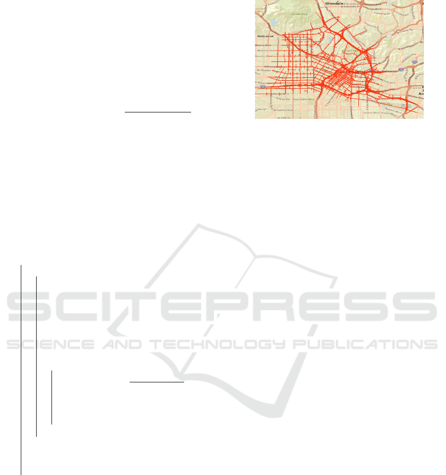
The real-life Los Angeles (LA) downtown network

shown in Figure 1 is a large-scale network composed

of 3,556 links (Abdelghaffar and Rakha, 2019). It is

characterized by congested trafﬁc, long travel times,

Figure 1: Downtown Los Angeles network.

and frequent delays. To alleviate the congestion, our

ultimate goal is to apply the network perimeter control

strategy in the congested region (Elouni et al., 2021).

For the control system to function properly, the area

where it will be implemented must exhibit homoge-

neous congestion. In other words, a densely homo-

geneous area that is geographically connected must

be located. Therefore, the GeoSOM algorithm is de-

ployed across the network, considering both the link

densities and their geographic locations, to achieve

this objective.

Every network link is characterized by two fea-

tures: its density (k), considered a non-geographical

feature, and its midpoint location, represented by x

and y coordinates, considered a geographical feature.

To prevent any feature from being weighted more than

the others, x, y, and k are normalized to values be-

tween 0 and 1.

Throughout the simulation, the neuron weights are

updated until they converge to a state where either the

change becomes minimal or ceases altogether. Then,

the distances between each neuron and its neighbor-

ing neurons are computed using the uniﬁed distance

matrix, commonly referred to as the U-matrix (Hamel

and Brown, 2011). Neurons are grouped into the same

clusters when the distances between them are rela-

tively small, while cluster boundaries are delineated

by larger distances between neurons. To deﬁne a color

code for each network link, the U-matrix results are

projected and interpolated into the input space. Based

on these colors, the clusters are then visually identi-

ﬁed.

4 SENSITIVITY ANALYSIS

The objective of this research is to identify a heavily

congested homogeneous area to manage congestion

within it. In evaluating GeoSOM’s effectiveness, our

emphasis was on identifying a speciﬁc area charac-

terized by a high volume of vehicles, i.e., high trafﬁc

Geographical Self-Organizing Map Clustering in Large-Scale Urban Networks for Perimeter Control

467

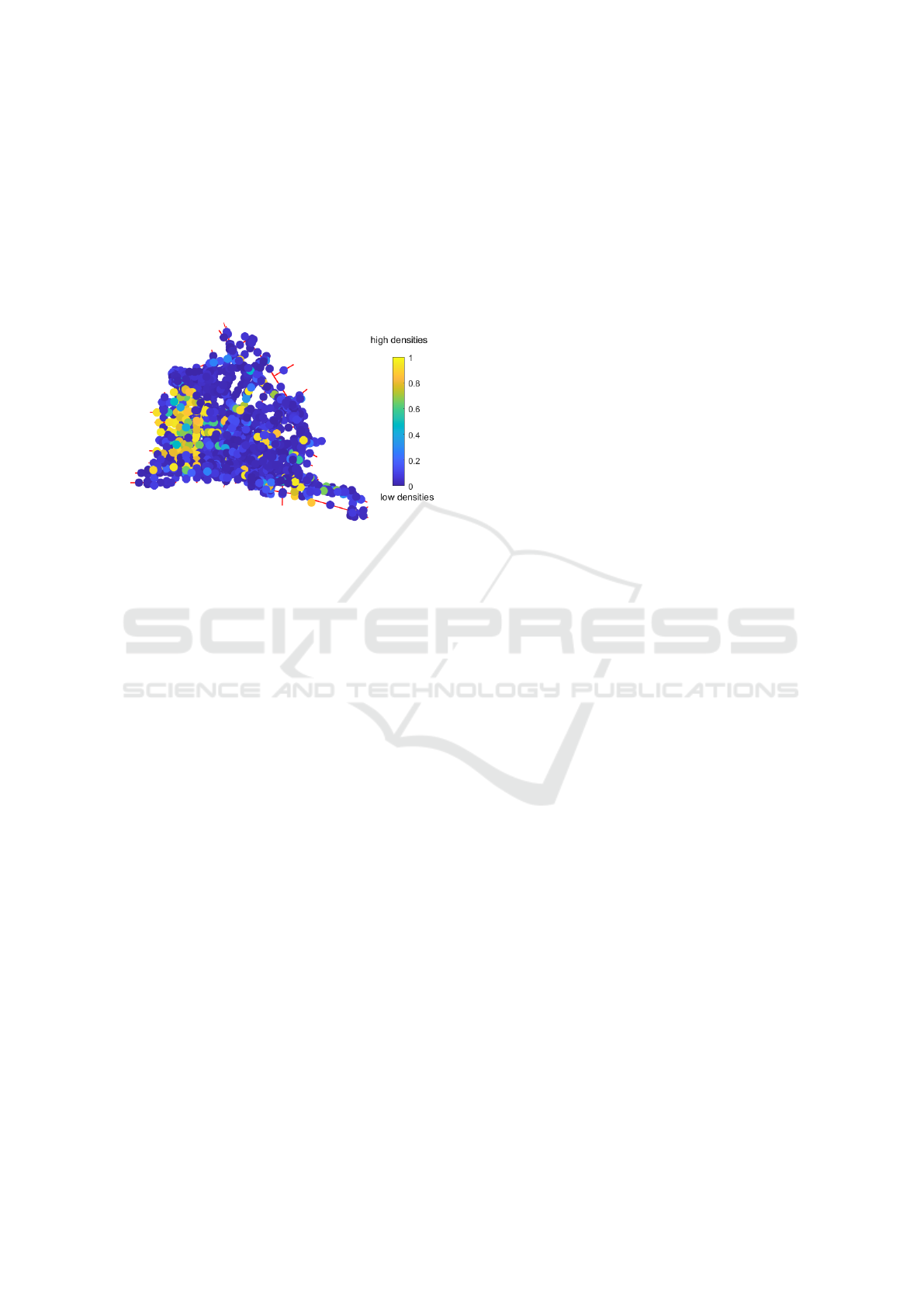
density. The peak density observed in the LA real

trafﬁc volume during rush hour is represented by the

yellow zone in Figure 2.

GeoSOM operates on artiﬁcial neural networks

and encompasses multiple parameters that necessi-

tate ﬁne-tuning. These parameters include the number

of neurons, the learning rate, and geographical toler-

ance. The best conﬁguration is determined through a

sensitivity analysis, as presented below.

Figure 2: LA real link densities.

4.1 Number of Neurons

GeoSOM was executed with varying numbers of neu-

rons, ranging from a 5×5 to a 25×25 grid, on the LA

network. Figure 3 depicts three cases, corresponding

to grid sizes of 5 × 5, 15 × 15, and 25 × 25, respec-

tively, from left to right.

Figure 3a illustrates the neurons’ grid at the end of

the simulation, following Algorithm 1. Meanwhile,

Figure 3b displays a color-coded interpolation of the

neurons’ weights onto the network links. Blue indi-

cates similar densities among the links, implying they

could potentially be clustered together, whereas yel-

low indicates a notable disparity in densities, imply-

ing they should not be clustered together. The left-

most plot in Figure 3a shows that the neurons did

not adequately cover the map, implying that a 5 × 5

neuron conﬁguration is inadequate. Furthermore, the

outcome for the 25 × 25 neuron conﬁguration, as de-

picted in Figure 3b, reveals that all the links are

grouped into only a single large cluster. Therefore,

25 × 25 neurons are ineffective. Figure 3 shows that

the best number of neurons is 15 × 15. The neuron

grid efﬁciently covers the network, as evidenced by

the middle plot in Figure 3a, and it also effectively

achieves homogeneous clusters, as indicated by the

dark blue color with clear light color boundaries in

the middle plot of Figure 3b.

4.2 Learning Rate

In this section, various learning rates (α) were exper-

imented within the GeoSOM algorithm. As α falls

between 0 and 1, the tested values ranged between

0.05 to 0.8. Figure 4 shows GeoSOM results for three

different α values. It is evident that for small α values

(e.g., α = 0.05), the homogeneous regions, character-

ized by a dark blue color, are quite small, which may

not be optimal for the control objective. Conversely,

with a high α value (e.g., α = 0.8), the network is

consolidated into a single cluster. The best α value

appears to be 0.4, where a well-deﬁned homogeneous

dark blue area is discernible with clear distinct bor-

ders, exhibited by yellow and green colors, making it

more suitable for control purposes.

4.3 Geographical Tolerance

This section investigates the impact of geographical

tolerance (R) on GeoSOM results, with low R values

indicating that geographical attributes are prioritized

and higher R values indicating a preference for non-

geographical attributes over geography. The R values

tested with the GeoSOM algorithm ranged between 0

and 8.

Figure 5 illustrates that for R = 0, the clustering

results did not yield a homogeneous dark blue area.

As R increases, the dark blue area expands. A well-

deﬁned cluster emerged when R = 5. However, as

the geographical tolerance increases to R = 8, cluster

borders start to blur, and all links are grouped into a

single cluster.

4.4 Sensitivity Analysis Conclusion

The best conﬁguration for the GeoSOM clustering al-

gorithm is identiﬁed as 15 × 15 neurons, α = 0.4, and

R = 5. Within the various homogeneous areas de-

picted by the dark blue color in Figure 6, the area of

primary interest is the one with the highest mean den-

sity, representing the most congested area, as illus-

trated in Figure 2, and depicted by the black contour

in Figure 6.

5 COMPARING GeoSOM TO

OTHER CLUSTERING

ALGORITHMS

In this Section, the GeoSOM algorithm is compared

with two other widely used clustering techniques:

DBSCAN and K-means, to evaluate its performance.

VEHITS 2024 - 10th International Conference on Vehicle Technology and Intelligent Transport Systems

468

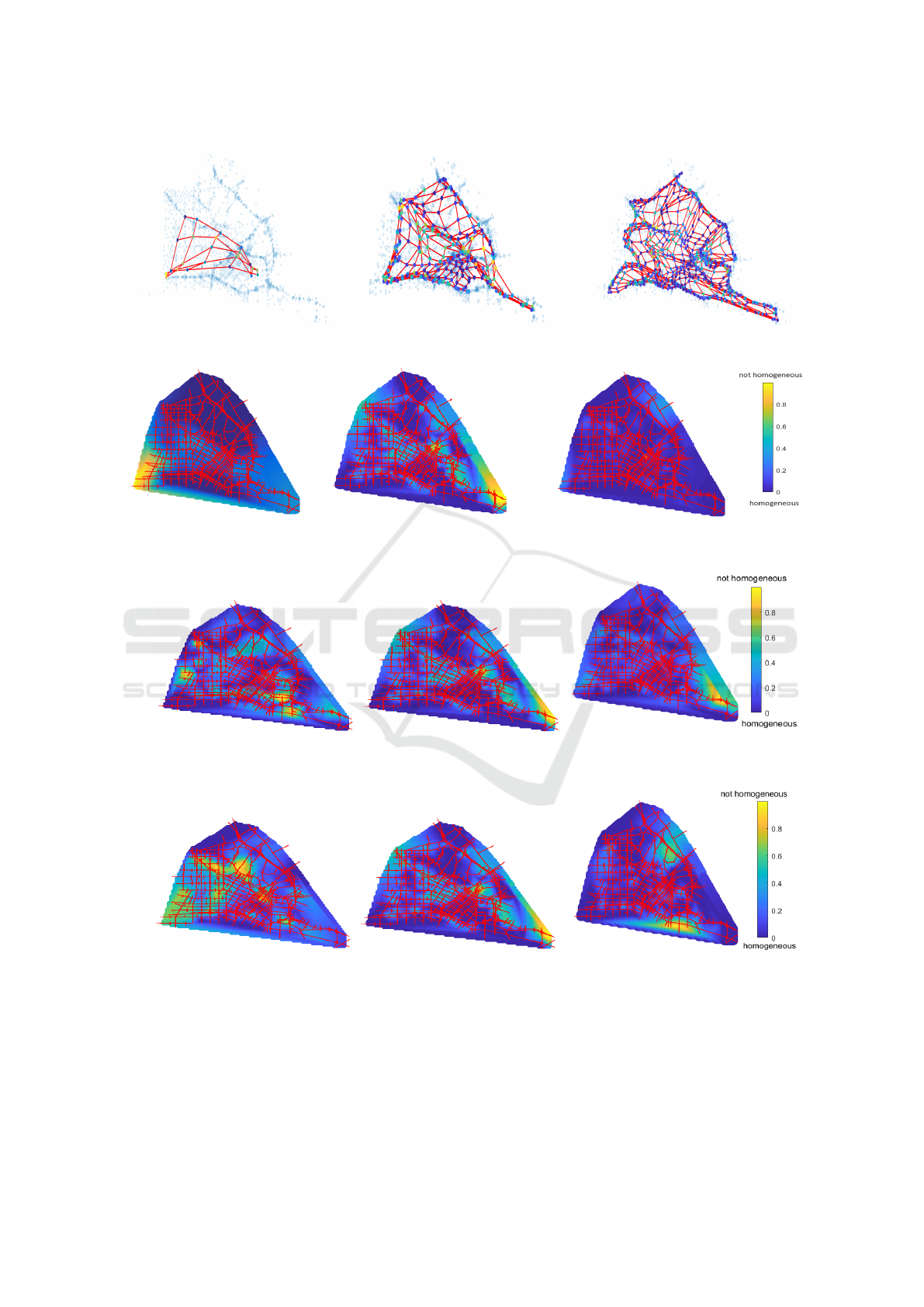
(a) Grid of neurons.

(b) Color-coded distances between the network links.

Figure 3: GeoSOM with different number of neurons; from left to right, 5 × 5, 15 × 15 and 25 × 25.

(a) α = 0.05. (b) α = 0.4. (c) α = 0.8.

Figure 4: GeoSOM maps for various α.

(a) R=0. (b) R=5. (c) R=8.

Figure 5: GeoSOM maps for various R.

While these two methods have been employed in the

literature for clustering transport networks, they lack

the explicit incorporation of geographical data, a fea-

ture inherent in GeoSOM (Lopez et al., 2017; Lin and

Xu, 2020).

5.1 DBSCAN

The density-based spatial clustering algorithm (DB-

SCAN) (Sahu et al., 2023) clusters points based on

their proximity to neighboring points. It relies on two

key parameters: ε, representing the radius of a neigh-

Geographical Self-Organizing Map Clustering in Large-Scale Urban Networks for Perimeter Control

469

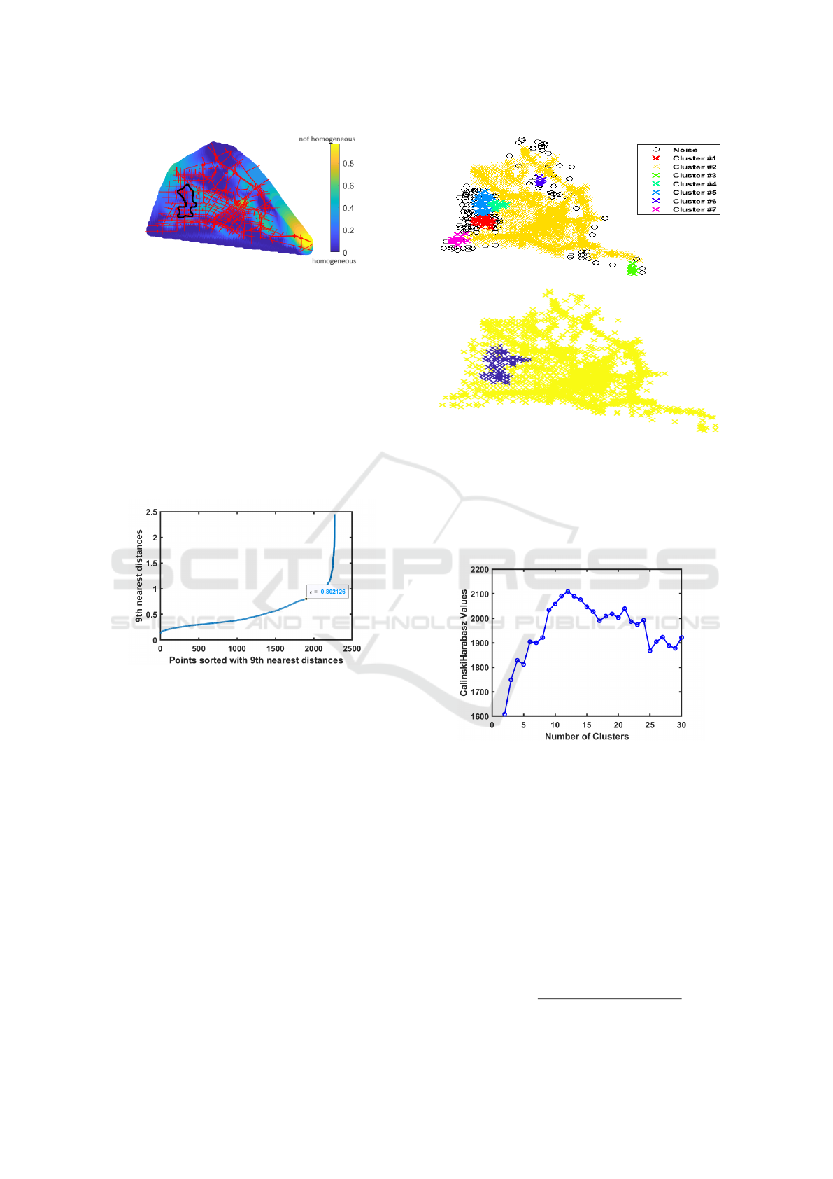
Figure 6: GeoSOM cluster identiﬁcation using best conﬁg-

uration.

borhood relative to a point, and minPts, which speci-

ﬁes the minimum number of points needed to consti-

tute a dense region, i.e., the minimum cluster size.

DBSCAN inputs are (x,y,k), where x and y rep-

resent geographical coordinates and k represents the

link density. DBSCAN’s sensitivity analysis utilizes

a k-distance graph to determine ε for each selected

minPts. The optimal values of ε are identiﬁed where

this graph exhibits an “elbow” as shown in Figure

7. Ultimately, the best parameters were found to be

minPts = 9 and ε = 0.8.

Figure 7: K-distance graph for DBSCAN.

Figure 8 shows the outcomes of the clustering

process. It is observed that clusters 1, 4, and 5 ex-

hibit high congestion levels and are geographically

connected based on the data in Figure 2. To facili-

tate comparison with the GeoSOM cluster, these three

clusters were merged. The combined cluster is illus-

trated in blue on the lower plot of Figure 8.

5.2 K-Means

K-means is a clustering algorithm that partitions data

points into k

clusters and assigns each point to the

cluster with the nearest mean. Often, it serves as a

benchmark to assess the performance of other cluster-

ing algorithms (Lopez et al., 2017; Saeedmanesh and

Geroliminis, 2016). Unlike DBSCAN, K-means only

requires the determination of one parameter, which is

the number of clusters.

The Calinski-Harabasz method (Aik et al., 2023)

Figure 8: DBSCAN.

is employed to identify the best number of clusters.

The results obtained using this method for k

values

ranging from 2 to 30 indicate that k

= 12 is the best

number of clusters, i.e., the maximum value in Figure

Figure 9: Calinski Harabasz for K-means.

The clustering outcomes are displayed in Figure

10, where cluster 12 corresponds to the most con-

gested area, as inferred from the data presented in Fig-

ure 2.

5.3 Performance Metrics

To evaluate the performance of the GeoSOM algo-

rithm, we compare it to the DBSCAN and K-means

algorithms using the following metrics:

• Quantization Error (QE):

QE =

||k(cluster) −

k(cluster)||

length(cluster)

VEHITS 2024 - 10th International Conference on Vehicle Technology and Intelligent Transport Systems

470

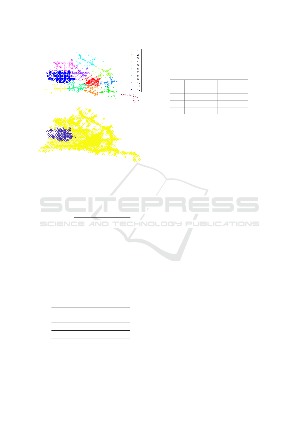
Figure 10: K-means.

where

k(cluster) represents the cluster’s mean

density, and length(cluster) represents the clus-

ter’s number of elements.

• Spatial Quantization Error (SQE):

SQE =

||xy(cluster) − ¯xy(cluster)||

length(cluster)

where ¯xy(cluster) represents the x and y coordi-

nates of the cluster’s centre.

• Density Variance (DV): It refers to the density

variance within the cluster, reﬂecting how much

the densities of individual points within the clus-

ter deviate from the mean density.

Table 1 illustrates the three performance metrics

for the three clustering algorithms. The performance

is improved when QE, SQE, and DV are minimized.

Table 1 demonstrates that GeoSOM outperforms the

other two algorithms.

Table 1: Performance metrics.

QE SQE DV

DBSCAN 0.0396 0.0095 0.1241

K-means 0.0333 0.0055 0.1494

GeoSOM 0.0336 0.0037 0.0837

Table 2 presents the percentage improvements of

GeoSOM over DBSCAN and K-means across vari-

ous performance metrics. The most signiﬁcant en-

hancements are observed in SQE and DV, aligning

with GeoSOM’s objectives of fostering spatially con-

nected links within clusters (yielding the best SQE)

and achieving clusters with minimal density variance.

Table 2: Improvement percentage (%).

GeoSOM GeoSOM

over DBSCAN over K-means

QE 15.15 -0.9

SQE 61.05 32.72

DV 32.55 43.98

The results reveal that the GeoSOM approach suc-

cessfully achieved the research goal of identifying

highly congested and geographically compact clusters

with low-density variance, surpassing DBSCAN and

K-means with improvement percentages reaching up

to 43% in DV, up to 61% in SQE, and up to 15% in

QE. These ﬁndings could ultimately be used for the

development of trafﬁc control systems aimed at alle-

viating congestion within the network.

6 CONCLUSION

In this research, a novel clustering algorithm is pro-

posed (GeoSOM) to identify densely congested and

spatially compact areas within transportation net-

works. This study provides valuable insights for de-

veloping effective trafﬁc control strategies to alleviate

trafﬁc congestion. The proposed clustering algorithm

is evaluated on a large-scale urban network in down-

town Los Angeles, and its performance is compared

to two other clustering algorithms, namely: DBSCAN

and K-means. The results demonstrated enhance-

ments across all three performance metrics when us-

ing GeoSOM compared to DBSCAN and K-means.

Speciﬁcally, there was a 15% reduction in the quan-

tization error, a reduction of up to 43% in the trafﬁc

stream density variance within the cluster, and a re-

duction of up to 61% in the spatial quantization er-

ror. The results also demonstrate GeoSOM’s effec-

tiveness in accurately delineating spatially homoge-

neous, congested areas within a large-scale network.

This research establishes a framework for harnessing

advanced clustering algorithms to tackle intricate traf-

ﬁc management challenges, thereby paving the way

for more efﬁcient urban mobility solutions. Future re-

search will involve leveraging this study’s ﬁndings to

develop network perimeter control strategies targeting

congested areas to reduce congestion and improve the

overall efﬁciency of urban transport systems.

Geographical Self-Organizing Map Clustering in Large-Scale Urban Networks for Perimeter Control

471

ACKNOWLEDGEMENTS

This work was partially funded by the Department of

Energy through the Ofﬁce of Energy Efﬁciency and

Renewable Energy (EERE), Vehicle Technologies

Ofﬁce, Energy Efﬁcient Mobility Systems Program

under award number DE-EE0008209. M. Elouni ac-

knowledges the receipt of the Chenery Grant from

Randolph-Macon College. M. Menendez acknowl-

edges the support of the NYUAD Center for Interact-

ing Urban Networks (CITIES), funded by Tamkeen

under the NYUAD Research Institute Award CG001.

REFERENCES

Abdelghaffar, H. M. and Rakha, H. A. (2019). A novel de-

centralized game-theoretic adaptive trafﬁc signal con-

troller: Large-scale testing. Sensors, 19(10).

Aik, L. E., Choon, T. W., and Abu, M. S. (2023). K-means

algorithm based on ﬂower pollination algorithm and

calinski-harabasz index. In Journal of Physics: Con-

ference Series, volume 2643, page 012019. IOP Pub-

lishing.

Bac¸

ao, F., Lobo, V., and Painho, M. (2004). Geo-self-

organizing map (geo-som) for building and explor-

ing homogeneous regions. In International Confer-

ence on Geographic Information Science, pages 22–

37. Springer.

Bac¸

ao, F., Lobo, V., and Painho, M. (2005). Geo-som and

its integration with geographic information systems.

In Proc. Workshop on Self-Organizing Maps, Paris,

France.

Bichiou, Y., Elouni, M., Abdelghaffar, H. M., and Rakha,

H. A. (2020). Sliding mode network perimeter con-

trol. IEEE Transactions on Intelligent Transportation

Systems, 22(5):2933–2942.

Elouni, M., Abdelghaffar, H. M., and Rakha, H. A. (2021).

Adaptive trafﬁc signal control: Game-theoretic decen-

tralized vs. centralized perimeter control. Sensors,

21(1):274.

Feng, Z., Xu, C., Zuo, Y., Luo, X., Wang, L., Chen, H.,

Xie, X., Yan, D., and Liang, T. (2023). Analysis of

water quality indexes and their relationships with veg-

etation using self-organizing map and geographically

and temporally weighted regression. Environmental

Research, 216:114587.

Hamel, L. and Brown, C. W. (2011). Improved inter-

pretability of the uniﬁed distance matrix with con-

nected components. In Proceedings of the Interna-

tional Conference on Data Science (ICDATA), page 1.

The Steering Committee of The World Congress in

Computer Science, Computer Engineering and Ap-

plied Computing (WorldComp).

Henriques, R., Bacao, F., and Lobo, V. (2012). Exploratory

geospatial data analysis using the geosom suite. Com-

puters, Environment and Urban Systems, 36(3):218–

232.

Kim, J.-Y., Gim, U. S., and Oh, M. T. (2014). Characteris-

tic analysis and classiﬁcation of rural areas: Based on

the eup and myon areas of chungcheongnam-do. The

Korean Regional Development Association, 26(1):27–

44.

Kim, T.-S., Dhakal, T., Kim, S.-H., Lee, J.-H., Kim, S.-

J., and Jang, G.-S. (2023). Examining village char-

acteristics for forest management using self-and geo-

graphic self-organizing maps: A case from the baek-

dudaegan mountain range network in korea. Ecologi-

cal Indicators, 148:110070.

Kohonen, T. (2013). Essentials of the self-organizing map.

Neural networks, 37:52–65.

Le Thi, H. A. and Nguyen, M. C. (2014). Self-organizing

maps by difference of convex functions optimiza-

tion. Data Mining and Knowledge Discovery, 28(5-

6):1336–1365.

Lin, X. and Xu, J. (2020). Road network partition-

ing method based on canopy-kmeans clustering algo-

rithm. Archives of Transport, 54(2):95–106.

Lopez, C., Krishnakumari, P., Leclercq, L., Chiabaut, N.,

and van Lint, H. (2017). Spatiotemporal partition-

ing of transportation network using travel time data.

Transportation Research Record, 2623(1):98–107.

Lukas Amb

uhl, Monica Menendez, M. C. G. (2023).

Understanding congestion propagation by combining

percolation theory with the macroscopic fundamental

diagram. Communications Physics, 6(26).

Melin, P., Monica, J. C., Sanchez, D., and Castillo, O.

(2020). Analysis of spatial spread relationships of

coronavirus (covid-19) pandemic in the world using

self organizing maps. Chaos, Solitons & Fractals,

138:109917.

Pires, F. J., Lobo, V., and Bac¸

ao, F. (2007). Insights on

the interpretation of som and u-matrices with an ex-

ample clustering based in oceanographic data. In 10th

AGILE international conference on geographic infor-

mation science, Aalborg University, Denmark.

Provenzano, D. and Giambrone, R. (2023). Clustering of

tourism patterns with self-organizing maps: The case

of sicily. Tourism Analysis.

Ran, X., Zhou, X., Lei, M., Tepsan, W., and Deng, W.

(2021). A novel k-means clustering algorithm with a

noise algorithm for capturing urban hotspots. Applied

Sciences, 11(23):11202.

Saeedmanesh, M. and Geroliminis, N. (2016). Clustering of

heterogeneous networks with directional ﬂows based

on “snake” similarities. Transportation Research Part

B: Methodological, 91:250–269.

Sahu, R. T., Verma, M. K., and Ahmad, I. (2023). Density-

based spatial clustering of application with noise ap-

proach for regionalisation and its effect on hierarchi-

cal clustering. International Journal of Hydrology Sci-

ence and Technology, 16(3):240–269.

Waters, N. (2017). Tobler’s ﬁrst law of geography. The

international encyclopedia of geography, pages 1–13.

Wulandari, V., Syarif, Y., Alﬁan, Z., Althof, M. A., and

Muﬁdah, M. (2024). Comparison of density-based

spatial clustering of applications with noise (dbscan),

k-means and x-means algorithms on shopping trends

data. IJATIS: Indonesian Journal of Applied Technol-

ogy and Innovation Science, 1(1):1–8.

VEHITS 2024 - 10th International Conference on Vehicle Technology and Intelligent Transport Systems

472