Optimising Data Processing in Industrial Settings: A Comparative

Evaluation of Dimensionality Reduction Approaches

Jos

e Cac¸

1,2 a

, M

ario Antunes

3,4 b

, Jos

e Santos

1,2 c

and Miguel Monteiro

TEMA, Centro de Tecnologia Mec

anica e Automac¸

ao, Departamento de Engenharia Mec

anica, Univerisdade de Aveiro,

3810-193 Aveiro, Portugal

LASI, Laborat

orio Associado de Sistemas Inteligentes, Guimar

aes, Portugal

DETI, Departamento de Eletr

onica, Telecomunicac¸

oes e Inform

atica, Universidade de Aveiro, Campus de Santiago,

3810-193 Aveiro, Portugal

IT, Instituto de Telecomunicac¸

oes, Aveiro, 3810-193 Aveiro, Portugal

Bosch Termotecnologia S.A., 3800-627 Cacia, Portugal

Keywords:

Dimensionality Reduction, IIoT, Feature Extraction, Feature Selection.

Abstract:

The industrial landscape is undergoing a signiﬁcant transformation marked by the integration of technology

and manufacturing processes, giving rise to the concept of the Industrial Internet of Things (IIoT). IIoT is

characterized by the convergence of manufacturing processes, smart IoT devices, and Machine Learning (ML)

algorithms, enabling continuous monitoring and optimisation of industrial operations. However, this evolution

translates into a substantial increase in the number of interconnected devices and the amount of generated data.

Consequently, with ML algorithms facing an exponentially growing volume of data, their performance may

decline, and processing times may signiﬁcantly increase. Dimensionality reduction (DR) techniques emerge

as a viable and promising solution, promoting dataset feature reduction and the elimination of irrelevant infor-

mation. This paper presents a comparative study of various DR techniques applied to a real-world industrial

use case, focusing on their impact on the performance and processing times of multiple classiﬁcation ML

techniques. The ﬁndings demonstrate the feasibility of applying DR: for a Logistic Regression classiﬁer, mi-

nor 4% performance decreases were obtained while achieving remarkable improvements, over 300%, in the

processing time of the classiﬁer for multiple DR techniques.

1 INTRODUCTION

Industry has recently undergone its 4

major revolu-

tion, Industry 4.0, marked by the widespread adop-

tion of technologies such as Machine Learning (ML),

Internet of Things (IoT), or Artiﬁcial Intelligence

(AI), and giving rise to the concept of Industrial In-

ternet of Things (IIoT). Furthermore, as industries

embrace Industry 4.0, a new industrial paradigm, In-

dustry 5.0, is currently unfolding (Xu et al., 2021).

While Industry 4.0 primarily focused on process

automation and optimisation, Industry 5.0 revolves

around a human-centric industrial environment, fos-

tering seamless collaboration between technology and

human resources. This collaboration strives to de-

https://orcid.org/0000-0002-4627-079X

https://orcid.org/0000-0002-6504-9441

https://orcid.org/0000-0003-0417-8167

velop more sustainable and environmentally friendly

industrial processes and solutions (Xu et al., 2021;

Maddikunta et al., 2022; Nahavandi, 2019). This new

paradigm, emphasising human-technology collabora-

tion and decentralised decision-making, outlines the

need for an even deeper intertwining of AI, ML and

IIoT to enhance ﬂexibility, adaptability, and efﬁciency

in industrial operations (Xu et al., 2021; Maddikunta

et al., 2022; Nahavandi, 2019).

In the pursuit for ﬂexible and efﬁcient industrial

processes, AI has emerged as a key player within

IIoT, facilitating processing tasks such as fault de-

tection and prediction, equipment health monitoring,

and predictive maintenance (Sisinni et al., 2018; An-

gelopoulos et al., 2020; Yao et al., 2017). However,

such tasks require substantial amounts of data; conse-

quently, the growth of IIoT has resulted in a signiﬁ-

cant increase in the amount of interconnected devices

generating data, a phenomenon commonly referred to

Cação, J., Antunes, M., Santos, J. and Monteiro, M.

Optimising Data Processing in Industrial Settings: A Comparative Evaluation of Dimensionality Reduction Approaches.

DOI: 10.5220/0012734000003705

Paper published under CC license (CC BY-NC-ND 4.0)

In Proceedings of the 9th International Conference on Internet of Things, Big Data and Security (IoTBDS 2024), pages 119-130

ISBN: 978-989-758-699-6; ISSN: 2184-4976

119

as Big Data (Hashem et al., 2015; Jia et al., 2022). De-

spite the robust capabilities of data-driven ML tools

in handling large datasets, the sheer volume of gen-

erated data can become overwhelming, adversely im-

pacting the performance of the ML algorithms, espe-

cially in time sensitive operations. The accumulation

of data not only introduces more variables into the

processes, but also brings in additional irrelevant and

redundant information, inadvertently leading to an in-

creasing process complexity.

In this context, Dimensionality Reduction (DR)

poses as a promising solution. Particularly for

data processing, having the possibility to reduce the

amount of features and dimensions of a given dataset

can prove advantageous for ML algorithms, reducing

the amount of data that is input to a classiﬁer or re-

gressor. As a result, the processing technique encoun-

ters a more streamlined dataset, enabling more efﬁ-

cient data processing. Furthermore, integrating DR

within an IIoT architecture can bring additional ben-

eﬁts, including data noise reduction, increased data

protection, and enhanced data storage and visualisa-

tion (Chhikara et al., 2020).

DR encompasses a set of techniques aimed at re-

ducing the dimension of a given dataset, while pre-

serving as much information as possible (Jia et al.,

2022). This reduction can be achieved through vari-

ous methods, whether by employing approaches that

ﬁlter and select a subset of the original features, re-

ferred to as Feature Selection (FS), or by generating

a new set of features that represent a mapping of the

original ones, termed Feature Extraction (FE). Us-

ing DR offers numerous beneﬁts, including reducing

the complexity of a given dataset, eliminating redun-

dant or irrelevant information, and contributing to a

faster and more efﬁcient processing of the informa-

tion for ML classiﬁers or regressors (Ayesha et al.,

2020; Huang et al., 2019). Owing to their ability

to decrease data volume and dataset complexity, DR

may play a crucial role in the rapidly evolving land-

scape of technology-connected industries.

In light of this, the main contributions of this pa-

per involve providing a comparative study, concern-

ing both performance and processing time analyses,

of several DR techniques applied to a dataset ob-

tained from a real-world industrial setting. The spe-

ciﬁc use case centres around a boiler testing proce-

dure conducted in the ﬁnal stages of a boiler pro-

duction line at Bosch Termotecnologia Aveiro

. Nu-

merous variables are captured during the testing pro-

cess, with the aim of determining the testing outcomes

based on the collected data. Seven commonly em-

https://www.bosch.pt/a-nossa-empresa/

bosch-em-portugal/aveiro/

ployed DR approaches, namely Principal Component

Analysis (PCA), Independent Component Analysis

(ICA), Non-negative Matrix Factorization (NMF),

Singular Value Decomposition (SVD), Random For-

est (RF), Recursive Feature Elimination (RFE), and

Autoencoder (AE) were analysed, employing also

four classiﬁers - Logistic Regression (LR), k-Nearest

Neighbours (kNN), RF, and Multi-layer Perceptron

neural network (MLP) - for a more comprehensive

evaluation. The ﬁnal ﬁndings illustrate that, for the

LR classiﬁer, signiﬁcant reductions in processing and

ﬁtting times (more than 300%) can be achieved at the

cost of only a 4% compromise in performance, using

techniques like PCA, SVD, and ICA.

The remainder of the paper is organised as fol-

lows. Section 2 provides a concise overview of DR

techniques and their main families/groups. Section 3

elucidates the main techniques and steps implemented

and incorporated in the comparative study. Section 4

presents and discusses the main ﬁndings of the com-

parative study. Finally, Section 5 provides the main

conclusions drawn, accompanied by suggested future

works.

2 BACKGROUND

DR techniques can be categorised into various classes

and subclasses, with the most common division being

between FE and FS. FE involves generating a new set

of features that represents a combination of the orig-

inal data, whereas FS consists of selecting a subset

of the original features (Jia et al., 2022; Zebari et al.,

2020). This section offers a brief introduction to DR,

delineating these multiple groups, and subsequently

emphasises the importance of applying DR in indus-

trial data processing.

2.1 DR Techniques

DR encompasses a set of techniques aimed at reduc-

ing the dimensions and simplifying a dataset. Given

the variety of approaches, they are commonly split

into multiple categories, the two main groups being

FS and FE. Some authors, such as Jia et al. (2022),

propose a third group - Deep Learning (DL) meth-

ods. Those can include both FE and FS, but leverage

neural network architectures to promote DR. Then,

various authors propose diverse subdivisions for DR

(Zebari et al., 2020; Solorio-Fern

andez et al., 2019;

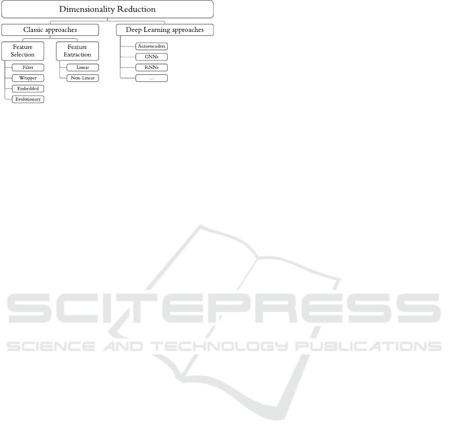
Ashraf et al., 2023). Drawing from these literature

proposals, Figure 1 presents a basic taxonomy outlin-

ing the primary families and subfamilies of DR.

IoTBDS 2024 - 9th International Conference on Internet of Things, Big Data and Security

120

Dimensionality Reduction

Classic approaches Deep Learning approaches

Feature

Selection

Feature

Extraction

Filter

Wrapper

Evolutionary

Embedded

Autoencoders

CNNs

RN N s

...

Linear

Non-Linear

Figure 1: Taxonomy of DR techniques, based on some lit-

erature proposals (Jia et al., 2022; Solorio-Fern

andez et al.,

2019; Zebari et al., 2020; Ashraf et al., 2023).

Feature Selection

FS techniques focus on reducing the dimensional-

ity of a dataset by selecting a subset of the initial

features, operating on the premise that these fea-

tures contain all essential information (Zebari et al.,

2020; Chhikara et al., 2020). FS is mainly split into

3 subclasses: ﬁlter, wrapper and embedded meth-

ods. Filter-based approaches rank features by im-

portance, deﬁning thresholds and rules determining

which variables to retain and which to discard (Jia

et al., 2022). Wrapper-based approaches are used

in conjunction with a classiﬁer, selecting a variable

group that maximises the performance of the classiﬁer

(Solorio-Fern

andez et al., 2019). Embedded methods

combine characteristics from ﬁlter and wrapper ap-

proaches, integrating a classiﬁer that adjusts its pa-

rameters iteratively according to the importance of

each feature (Zebari et al., 2020). An additional ap-

proach involves evolutionary methods, e.g., Genetic

Algorithm or Particle Swarm Optimisation, to select

an optimal feature set.

FS offers advantages such as keeping the original

physical signiﬁcance of data (as no data transforma-

tion is applied), while preserving interpretability (Ze-

bari et al., 2020; Jia et al., 2022). However, the trade-

off between number of features and data relevance

needs to be handled carefully, as large reductions may

lead to loss of relevant information.

Feature Extraction

The objective of FE is to create a new set of features,

or components, mapping the initial set of variables

(Jia et al., 2022; Zebari et al., 2020). FE can be mainly

categorised into two subclasses, linear and non-linear

methods. This distinction is based on whether they

consider the linearity of data. Linear approaches as-

sume that the new feature set forms a linear mapping

of the original one, i.e., the lower-dimension repre-

sentation is a linear combination of the original fea-

tures (Anowar et al., 2021). However, linear meth-

ods may fail to capture true non-linear relationships

within data if the original data is non-linear and ex-

hibits dependencies between variables. Conversely,

non-linear techniques can be employed to capture the

more intricate dependencies within non-linear data

(Chhikara et al., 2020).

Applying FE provides the potential for a smaller

set of reduced features when compared to FS. The re-

duced data, being a combination of the original data,

retains the dependencies of the initial dataset, facil-

itating more efﬁcient removal of redundant informa-

tion (Zebari et al., 2020; Jia et al., 2022). However,

the application of FE comes with the drawback of data

loss of interpretability and physical meaning.

DL-Based Approaches

DL-based approaches leverage neural networks, par-

ticularly in FE tasks. Various techniques can be used

to extract the most relevant information and features

from data. For instance, Recurrent Neural Networks

(RNNs), like Long Short-Term Memory (LSTM) and

Gated Recurrent Units (GRU), are utilised to extract

sequential and time-dependent features from data.

Convolutional Neural Networks (CNNs) are effective

in extracting spatial features, commonly applied to

process image data. Another notable DL-based ap-

proach are AEs, notable for their architecture. As il-

lustrated in Figure 2, they consist of an encoder, a de-

coder, and a latent space representation. They aim at

discovering a compressed representation of the origi-

nal data through the encoder, and then reconstructing

it back to its original state via the decoder. This design

forces the AE to learn the most important features in

data resulting in a lower-dimensional representation

in the latent space. Additionally, depending on the

scope of the problem, different neural network layers

can be employed within the AE to extract temporal,

sequential, spatial, among other features.

2.2 DR Importance Within Industrial

Environments

As previously highlighted in Section 1, the indus-

trial paradigm is currently shifting towards the inte-

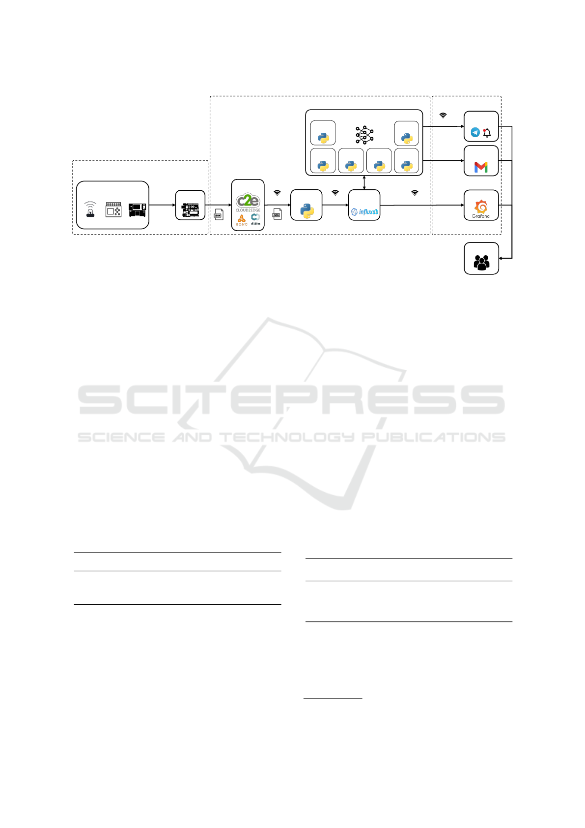
gration of new technologies. IIoT architectures, such

as the one depicted in Figure 3, are adopting a lay-

ered and block-structured design. In this evolving

IIoT paradigm, key processes include data gathering,

transfer, storage, processing, and visualisation. En-

suring a rapid and secure data ﬂow between these

blocks is crucial, especially for applications that de-

mand low-latency processing and response times.

In architectures of this kind, the proliferation of

Optimising Data Processing in Industrial Settings: A Comparative Evaluation of Dimensionality Reduction Approaches

121

Input

Layer

Latent

Space

ˆx

Output

Layer

Figure 2: Base architecture of an autoencoder.

IoT sensing devices near the manufacturing processes

has resulted in an impressive increase in the volume of

collected data. Consequently, there is a growing need

to process the data via ML algorithms. While having

more data about manufacturing processes is advanta-

geous and facilitates a more profound understanding,

it also introduces challenges within the IIoT frame-

work. The increased data quantity poses challenges

in terms of data transmission, resulting in higher la-

tencies. Data storage systems may become more

congested, leading to reduced storage space. Visu-

alising and understanding relationships among var-

ious process variables can become more challeng-

ing due to the abundance of information. Moreover,

data processing is also affected, as more data inadver-

tently leads to more redundant and irrelevant informa-

tion, possibly decreasing the performance of the al-

gorithms. Additionally, larger amounts of data trans-

late into larger processing times, potentially impair-

ing response times and the ability of the architecture

to promptly handle data (Ashraf et al., 2023; Jia et al.,

2022).

DR emerges as a promising solution to address

these challenges, particularly in the context of data

processing. Its main positive impact is evident when

applied as a pre-processing step for ML classiﬁers or

regressors, effectively eliminating redundant and ir-

relevant information, and thereby improving process-

ing time and performance outcomes for the ML tech-

niques. One such example is the work of G

omez-

Carmona et al. (2020), who demonstrated that the

application of DR techniques achieved, for their use

case, an 80% reduction in computational efforts and

time, with only a 3% decline in ML model perfor-

mance. However, DR not only proves beneﬁcial for

data processing. Other potential advantages of its im-

plementation may be the following:

• Enhancing Data Storage: reducing data entering

databases alleviates communication latencies and

conserves storage space;

• Improved Data Visualisation: by minimising

variables and irrelevant information, identifying

correlations in manufacturing processes variables

becomes more straightforward;

• Noise Reduction and Data Security: DR dimin-

ishes data noise. Therefore, less information is

transferred across the architecture, lowering the

risk of data leaks and possible cyberattacks.

3 METHODS

As previously mentioned, this paper exposes a com-

parative study of multiple DR techniques applied to

an industry-related dataset. The use case involves a

watertightness boiler testing process, conducted at the

end of the boilers’ production line, aiming to iden-

tify leaks within the piping systems. This constitutes

a multi-label classiﬁcation problem, with the target

variable indicating pass or fail outcomes for different

boilers. All testing code was developed in Python,

and is publicly accessible on GitHub

. This section is

dedicated to provide the main details about the testing

procedure.

3.1 Use Case and Dataset Description

Bosch Termotecnologia Aveiro, part of the Robert

Bosch GmbH

group, specialises in the production

of heat water solutions, primarily boilers and heat

pumps. This factory is one of Portugal’s most innova-

tive industrial environments, focused on the digitali-

sation and automation of their production lines, aim-

ing to enhance productivity and environmental efﬁ-

ciencies. Particularly, one of their main projects, IL-

LIANCE

, focuses on developing efﬁcient and sus-

tainable heating technologies, particularly hybrid gas

and hydrogen systems. Furthermore, there is also a

major focus on the digitalisation and improvement of

their productive building process.

In the ﬁnal stages of boiler production, each unit

undergoes a watertightness test to identify leaks and

deﬁciencies in the piping system. The test monitors

https://github.com/zemaria2000/DR Comparison

https://www.bosch.com/

https://www.illiance.pt/pt-pt

IoTBDS 2024 - 9th International Conference on Internet of Things, Big Data and Security

122

USER LAYER

DIGITAL LAYER

PHYSICAL LAYER

Shop ﬂoor

equipment

Sensors

PLCs CNCs

Gateway(s)

Cloud2Edge

MQTT

USER

SMTP

TCP/IP

Rs485

Modbus

…

Warnings +

Alerts

Data Mining

Intelligent Assistant

Model

building

HTTP

SSE

Client(s)

Database

HTTP HTTP

HTTP

Predicting

agent

Anomaly

detection agent

Report

building

Data

pre-processing

Notiﬁcation

generation

Reports

Visualisation

Figure 3: IIoT architecture used on a previous project (Cac¸

ao et al., 2024).

variables such as gas ﬂows, temperatures, and pres-

sures. If the values all fall within certain appropri-

ate intervals, the equipment passes the test, other-

wise, it fails it, and inadvertently halts the produc-

tion line. These test failures require manual exami-

nation, contributing to inefﬁciencies and production

bottlenecks. Within this scenario, DR can play a cru-

cial role in optimising the testing process, aiding in

selecting relevant features, for instance, and identify-

ing signiﬁcant variables, consequently enhancing ML

techniques’ processing efﬁciency.

The main characteristics of the described process

dataset are presented in Table 1. It comprises a total

of 48 variables, collected during each watertightness

test. The test results in a multi-label four class clas-

siﬁcation problem: two equipment classes, split into

successful and unsuccessful tests. The dataset is rela-

tively small, with 11962 samples in total, each repre-

senting the average values for each feature for a com-

plete testing procedure.

Table 1: Dataset description.

No. of

Features

No. of

Classes

Classes Samples

48 4

0: ’Equipment 1 - Failed’ 410

1: ’Equipment 1 - Passed’ 6372

2: ’Equipment 2 - Failed’ 390

3: ’Equipment 2 - Passed’ 4790

3.2 Pre-Processing Steps

To prepare data for the comparative study, several pre-

processing steps were employed to ensure a better

testing procedure. The main ones are outlined below:

1. Data Imputation: the original dataset, collected

at Bosch’s production environment, contained

missing values in some columns. To facilitate

processing by both DR techniques and classiﬁers,

data imputation was performed: NaN and Null

values were replaced by the mean value of their

respective column;

2. Data Balancing: as indicated in Table 1, the dis-

tribution of passed and failed tests is quite im-

balanced, with passed tests accounting for around

93% of the dataset. This imbalance can lead to

classiﬁer overﬁtting during training, potentially

negatively impacting testing performances. To ad-

dress this, a combination of SMOTE (Synthetic

Minority Oversampling Technique) and Tomek

Links was employed for data balancing (Swana

et al., 2022). SMOTE was used to oversample mi-

nority classes, while Tomek Links balanced the

undersampling of majority classes. This synthetic

data generation was carefully conducted, aiming

for a balanced 4:1 ratio of successful to unsuc-

cessful tests. The ﬁnal sample amounts are pre-

sented in Table 2;

Table 2: Number of samples for each class after data bal-

ancing using SMOTE and Tomek Links.

Classes

Original

Samples

Balanced

Samples

0: ’Equipment 1 - Failed’ 410 2124

1: ’Equipment 1 - Passed’ 6372 6370

2: ’Equipment 2 - Failed’ 390 1596

3: ’Equipment 2 - Passed’ 4790 4790

3. Data Normalisation: given the substantial dis-

crepancies in certain features’ values, data nor-

malisation was conducted using two scikit-learn

Python library scalers: ‘StandardScaler’, scaling

the data to have a mean of 0 and standard devia-

https://scikit-learn.org/stable/

Optimising Data Processing in Industrial Settings: A Comparative Evaluation of Dimensionality Reduction Approaches

123

tion of 1, and ‘MinMaxScaler’, scaling data to the

0-1 range. The latter was employed for methods

like NMF, unable to handle negative values.

4. Label Encoding: as exposed in both Table 1 and

Table 2, the original test labels consist of strings

indicating the equipment type and test result. To

facilitate the reading of output results by the ML

classiﬁers during training, label encoding was im-

plemented, creating integer labels for each distinct

class.

3.3 Testing Procedure

Following data pre-processing and preparation, a

comprehensive comparative testing procedure was

conducted utilising multiple DR techniques and clas-

siﬁers. The study, completely implemented in Python,

employed the scikit-learn and TensorFlow

libraries

for building the DR models. All classiﬁers were also

from the scikit-learn library, and were used with their

default hyperparameters, as well as most DR tech-

niques. Only to address convergence issues encoun-

tered during the ﬁtting process, adjustments were im-

plemented speciﬁcally for the ICA and NMF tech-

niques: the convergence tolerance, initially set by de-

fault at 1 × 10

−4

was changed to 5 × 10

−2

. Addition-

ally, the number of maximum iterations was adjusted

from the default value of 200 to 5000 and 10000 for

the ICA and NMF techniques, respectively. The AE,

the only method from the TensorFlow library, had the

following implementation details: a base architecture

comprised of layers with 48 (input dimension), 32,

16, 8, 4, and 2 nodes, ‘swish’ as the activation func-

tion, ‘adam’ as the optimiser, and mean squared error

as the loss function, evaluating the reconstruction er-

ror. Following ﬁtting, the encoder was extracted and

used to output the reduced data representation.

For both DR techniques and ML classiﬁers, 80%

of the datasets were used for training, 10% of those

for validation, and the remaining 20% to conduct the

tests. All tests were ran on the same machine, whose

characteristics are exposed in Table 3. Furthermore,

Table 4 exposes the Python and main used libraries’

versions.

Table 3: Main characteristics of the machine where the test

were conducted.

Processor

Base clock

speed

RAM Graphics card

AMD Ryzen 9

7950X 16-Core

Processor

4.5 GHz 128 GB

Nvidia GeForce

RTX 4090

https://www.TensorFlow.org/

Table 4: Python and main used libraries’ versions.

Library Version

Python 3.10.8

scikit-learn 1.3.2

TensorFlow 2.10.0

pandas 2.2.0

numpy 1.26.4

matplotlib 3.8.0

exectimeit 0.1.1

The tests conducted and discussed in Section 4 in-

clude:

• Assessing the inﬂuence of different DR ap-

proaches with varying numbers of reduced fea-

tures on classiﬁer performance;

• Evaluating classiﬁer ﬁtting and prediction times

for different dataset dimensions;

• Assessing ﬁtting and dataset reduction times for

some DR techniques.

The primary metric for evaluating model per-

formance was the Matthew’s Correlation Coefﬁcient

(MCC), calculated using the confusion matrix indica-

tors - True Positives (TP), True Negatives (TN), False

Positives (FP) and False Negatives (FN). The formula

is presented in Equation 1,

MCC =

TN × TP −FN × FP

(TP + FP)(TP +FN)(TN + FP)(TN + FN)

, (1)

with MCC ranging between -1 and 1. An MCC of

-1 indicates “perfect” misclassiﬁcation, an MCC of

1 perfect classiﬁcation, and an MCC of 0 indicates

predictions equivalent to random chance.

Finally, the measured times included ﬁtting times

for DR techniques and classiﬁers, prediction times for

the classiﬁers, and dataset reduction times for the DR

approaches. The exectimeit

library was used for time

measurements, following the work from Moreno and

Fischmeister (2017).

4 RESULTS AND DISCUSSION

This comparative study, as already mentioned, delved

into the performance and time impacts of employing

various DR techniques within an industrial real-world

dataset. This section outlines the key ﬁndings from

the conducted tests.

4.1 Performance Analysis

The initial test focused on evaluating the MCC for

various numbers of reduced components obtained

https://pypi.org/project/exectimeit/

IoTBDS 2024 - 9th International Conference on Internet of Things, Big Data and Security

124

with different DR techniques, and four distinct clas-

siﬁers. For non-DL methods, reduced dimensions

ranging from 2 to 47 were tested, while for the AE,

the reduced dimensions corresponded to the AE ar-

chitecture deﬁnition, 2, 4, 8, 16, and 32, i.e., each

test involved eliminating the previous last layer. Ta-

ble 5 and Table 6 present the MCC results for some

selected reduced dimensions and the MCC using the

entire dataset, respectively.

Table 5: Performance (MCC) comparisons between the DR

techniques, for all classiﬁers and for multiple reduced di-

mensions (at bold the best result for each DR technique,

underlined the values that outperformed the default tests).

DR Dim. LR kNN RF MLP

PCA

2 0.932 0.938 0.930 0.932

5 0.931 0.936 0.935 0.939

10 0.934 0.955 0.954 0.951

20 0.949 0.958 0.962 0.951

30 0.958 0.961 0.962 0.955

40 0.968 0.961 0.970 0.971

ICA

2 0.929 0.936 0.933 0.936

5 0.927 0.934 0.936 0.942

10 0.933 0.948 0.953 0.953

20 0.949 0.949 0.962 0.948

30 0.956 0.951 0.964 0.952

40 0.968 0.966 0.971 0.973

NMF

2 0.883 0.972 0.964 0.970

5 0.884 0.959 0.963 0.971

10 0.883 0.940 0.970 0.977

20 0.861 0.936 0.964 0.974

30 0.895 0.975 0.969 0.978

40 0.884 0.959 0.976 0.978

2 0.950 0.950 0.950 0.950

5 0.966 0.965 0.966 0.965

10 0.966 0.960 0.966 0.966

20 0.971 0.962 0.978 0.979

30 0.970 0.961 0.972 0.978

40 0.970 0.964 0.973 0.980

RFE

2 0.971 0.968 0.973 0.978

5 0.974 0.969 0.974 0.979

10 0.970 0.951 0.974 0.979

20 0.969 0.963 0.973 0.979

30 0.971 0.968 0.973 0.980

40 0.969 0.952 0.976 0.982

SVD

2 0.932 0.938 0.930 0.934

5 0.931 0.937 0.935 0.941

10 0.936 0.954 0.954 0.951

20 0.949 0.958 0.960 0.952

30 0.958 0.961 0.965 0.956

40 0.968 0.961 0.974 0.974

2 0.836 0.928 0.896 0.934

4 0.919 0.965 0.920 0.973

8 0.932 0.976 0.922 0.978

16 0.929 0.979 0.918 0.980

32 0.939 0.980 0.940 0.979

Table 6: MCC values for the 4 classiﬁers, using all available

features from the original dataset.

LR kNN RF MLP

0.946 0.974 0.990 0.974

Analysing the MCC values for the original dataset

(Table 6), all classiﬁers exhibited high performances,

with MCC values larger than 0.9. LR had the low-

est score, 0.946, with the highest belonging to the RF

classiﬁer, with 0.99.

Turning to the DR techniques (Table 5), it is evi-

dent that MCC values remain consistently high, with

most MCC scores above 0.9, even with very low-

dimensional datasets. Apart from the RF classiﬁer,

which achieved an MCC of 0.99 with the original

datasets, all other classiﬁers, combined with various

DR techniques, achieved higher performance metrics

with datasets with fewer features. Notable examples

include PCA with 20 components combined with LR,

resulting in an MCC of 0.949, compared to the origi-

nal value of 0.946; using an AE reducing the dataset

to just 16 features combined with the kNN classiﬁer,

obtaining an MCC of 0.979, surpassing the original

kNN test with 0.974; or using NMF with 30 features

and an MLP classiﬁer, achieving an MCC of 0.978,

opposed to the original 0.974.

For FE methods, PCA, ICA, NMF, SVD and AE,

there seems to be a tendency for improved perfor-

mances with a larger number of reduced components,

with more components being able to encode more in-

formation and retain more data dependencies. Con-

versely, FS methods, RF and RFE, showcase a much

more balanced performance, successfully identifying

two or ﬁve features that retain essential information

about the original dataset. Figure 4 visually illus-

trates this trend. ICA (Figure 4a) exhibits a clear per-

formance upward trend, for all classiﬁers, with the

MCC constantly increasing with the number of re-

duced components. Conversely, RFE (Figure 4b) re-

mains more horizontally stable, achieving very high

MCC values with very few features. This may sug-

gest that FS methods can efﬁciently identify a very

small set of features containing most essential in-

formation for classiﬁcation purposes, while FE tech-

niques struggle in creating a compact group of vari-

ables that excludes the irrelevant information.

In summary, the use of DR techniques speciﬁcally

for the use case explored did not seem to signiﬁcantly

inﬂuence classiﬁer performance. It was possible to

achieve quite high performances with a much smaller

dataset. Furthermore, in some cases, DR techniques

effectively discarded irrelevant and redundant infor-

mation, leading to classiﬁer performance improve-

ments. FS techniques, in particular, demonstrated a

Optimising Data Processing in Industrial Settings: A Comparative Evaluation of Dimensionality Reduction Approaches

125

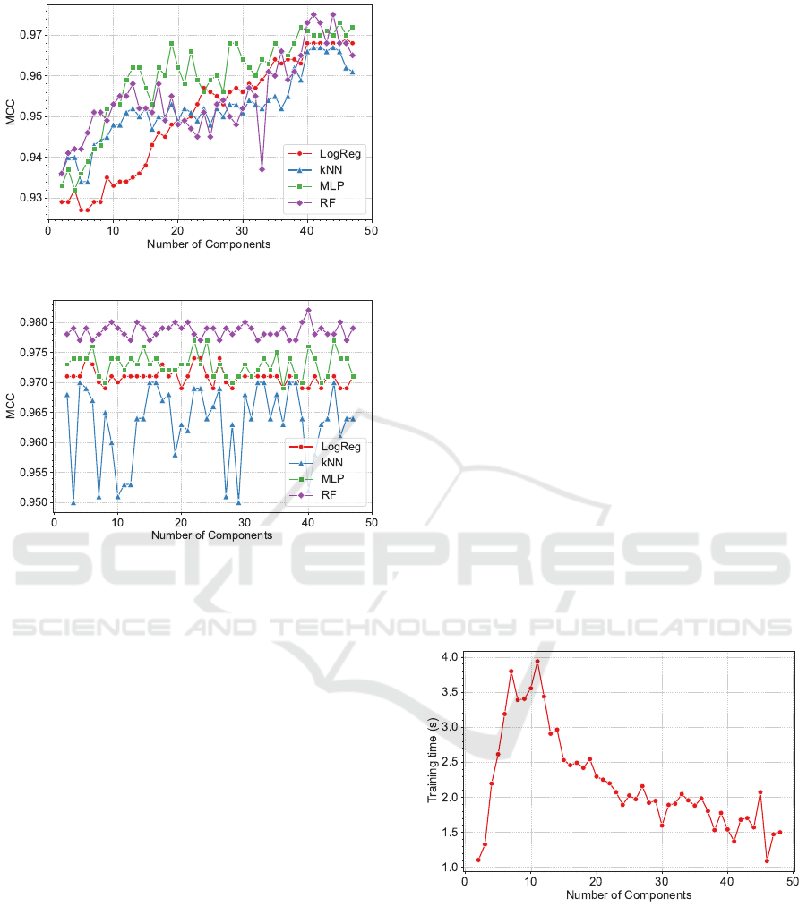
(a) ICA.

(b) RFE.

Figure 4: MCC for the 4 different classiﬁers, in the testing

dataset, depending on the number of components reduced

by the (a) ICA and (b) RFE DR techniques.

notable ability to select a small set of the original fea-

tures, outperforming FE techniques. Hence, for the

studied use case, DR methods emerge as promising

strategies, as despite utilising a signiﬁcantly reduced

set of features, the classiﬁer’s performance remains

quite high and satisfactory. Subsequent sections will

provide insights regarding the time beneﬁts of using

DR, reducing training and prediction times.

4.2 Classiﬁers Time Tests

As discussed earlier, an excessive number of variables

in a dataset may lead to longer ﬁtting and prediction

times for ML methods. Therefore, it is relevant to

assess the impact of applying DR in the ﬁtting and

prediction times of ML classiﬁers.

For this test, training and prediction times for the

four selected classiﬁers were assessed with different

reduced dataset sizes by each DR approach. To ac-

curately evaluate these times, each test (i.e., each re-

duced dataset from each DR technique, for each clas-

siﬁer) was conducted ﬁve times, using a dedicated

Python library, exectimeit. The complete test results

can be consulted in Table 10, in the Appendix section.

For this particular discussion, training and prediction

times for the ICA technique are presented in Table 7,

with the last row representing the times for the origi-

nal dataset.

Analysing the results in Table 7, particularly for

the LR and RF classiﬁers, there is a clear tendency

of increasing training and prediction times for larger

datasets. Larger datasets induce more data for the

models to process, resulting in longer training times.

For both these classiﬁers, the 40-feature datasets ex-

hibit approximately 5x longer training times com-

pared to the 2-feature datasets, consistent with expec-

tations. For prediction times, this growing tendency

is much less evident, but that would be expected, as

testing datasets are much smaller and the models are

already ﬁt.

However, for the kNN and the MLP classiﬁers, the

time tendencies differ. For kNN, there is a notable dif-

ference between training and prediction times, with

the latter being larger. This results from the kNN

prediction process, which requires distance calcula-

tions for each testing point, to each of its k-nearest

neighbours. Moreover, for both classiﬁers, the train-

ing times initially increase with the number of re-

duced components, and then signiﬁcantly decrease

with larger datasets. This behaviour might be due to

possible classiﬁer overﬁtting, resulting in faster con-

vergence times. Figure 5 further illustrates this differ-

ent time evolution for the MLP classiﬁer.

Figure 5: Training time evolution for the MLP classiﬁer

with the reduced ICA dataset.

Comparing reduced datasets with the original

ones, it is evident that in general, both training and

prediction times are larger for the full set of variables

compared to reduced datasets, as expected. This dif-

ference is substantial in some cases, namely for LR

and MLP. For LR, the ﬁtting time with the reduced

dataset is around 3x smaller than with the original

IoTBDS 2024 - 9th International Conference on Internet of Things, Big Data and Security

126

Table 7: Average training and prediction times for 5 runs, for multiple classiﬁers using the reduced datasets from the DR

techniques.

DR Dim.

LR kNN RF MLP

Train (ms) Pred (ms) Train (ms) Pred (ms) Train (ms) Pred (ms) Train (ms) Pred (ms)

ICA

2 14.20 ± 0.04 0.06 ± 0.01 2.22 ± 0.08 30.21 ± 0.27 1011.60 ± 12.96 13.29 ± 0.30 1103.64 ± 121.13 0.57 ± 0.04

5 18.82 ± 0.18 0.06 ± 0.01 3.57 ± 0.06 38.52 ± 0.29 1781.73 ± 27.85 12.92 ± 0.42 2612.49 ± 1224.58 0.78 ± 0.23

10 27.26 ± 0.10 0.06 ± 0.01 5.75 ± 0.08 111.47 ± 0.95 2773.43 ± 39.29 12.33 ± 0.26 3554.07 ± 817.27 0.82 ± 0.18

20 70.78 ± 0.46 0.08 ± 0.02 0.39 ± 0.08 6.80 ± 2.25 3892.33 ± 82.45 12.99 ± 0.39 2294.17 ± 259.82 0.77 ± 0.11

30 86.66 ± 1.59 0.19 ± 0.02 0.39 ± 0.11 10.25 ± 0.20 5523.99 ± 98.59 14.58 ± 0.52 1594.72 ± 358.41 0.83 ± 0.09

40 71.82 ± 1.96 0.19 ± 0.03 0.41 ± 0.09 8.43 ± 4.28 5296.30 ± 161.25 11.53 ± 0.56 1539.47 ± 616.59 0.77 ± 0.16

Default 48 283.21 ± 34.84 1.24 ± 0.36 3.24± 0.85 117.59 ± 74.71 2994.67 ± 208.77 16.82 ± 0.59 15123.26 ± 4476.46 2.62 ± 0.48

data (86.66ms opposed to 283.21ms). For the MLP

classiﬁer, the training times are 4x smaller (3.55s for

a 10-variable dataset opposed to more than 15s for the

original data).

Overall, the implementation of DR techniques sig-

niﬁcantly reduces ﬁtting and prediction times for clas-

siﬁers. While the differences may not be substantial

for this particular use case, with a small dataset com-

prised of less than 15000 samples and just 48 vari-

ables, it is important to note that in datasets with mil-

lions of samples and hundreds or thousands of vari-

ables, the reductions would be much more signiﬁcant

and with more pronounced impacts.

4.3 DR Techniques Time Tests

While testing the ﬁtting and prediction times of clas-

siﬁers is crucial for assessing the time beneﬁts of

reducing the number of variables in datasets, it is

equally relevant to evaluate the time required by the

DR approaches to train themselves and reduce the

datasets. If the time needed for training or generating

the reduced dataset is is excessively large, it becomes

highly inefﬁcient and even counterproductive to use

such techniques in combination with ML classiﬁers.

The purpose of DR techniques is to alleviate the clas-

siﬁers’ process times, and if DR takes too long, the

resulting time impacts may offset the beneﬁts, with

the additional cost of potential loss in classiﬁer per-

formance. Table 8 presents, for some DR techniques,

their training and reduction times for varying numbers

of features.

Examining the results in Table 8, PCA stands

out as the fastest technique in terms of both ﬁtting

and reduction times. The longest ﬁtting time is just

33.37ms, with reduction times mostly below 1ms.

Furthermore, NMF also showcases short training and

reduction times, with the longest being for the 32

component dataset, at 92.63ms, while reduction times

are in most cases smaller than 5ms. On the other hand,

using the encoder from an AE for DR induces sig-

niﬁcantly longer processing times: the largest train-

ing and reduction times are 11.3s and 93.42ms, sub-

stantially higher than those for the previous two tech-

niques. Moreover, the times tend to decrease with the

increase in the number of reduced features. This is

due to the base architecture and methodology used for

the AE tests, with the largest autoencoder (i.e., with

the most layers) achieving the largest dimension re-

duction.

In conclusion, as highlighted earlier, it is crucial

to consider both the time beneﬁts of reducing the

datasets for classiﬁers, and the training and reduction

times of the DR techniques themselves. As shown,

using DL-based techniques may lead to consider-

able training and even reduction times, and this fac-

tor should be considered, especially in time-sensitive

operations when applying DR in conjunction with a

classiﬁer.

4.4 Overall Performance and Time

Comparison

As discussed throughout this results section, the use

of DR techniques can offer beneﬁts in both perfor-

mance and processing time, particularly for time-

sensitive industrial processes, and it is crucial to ﬁnd

the right balance between performance and dataset

size. This ﬁnal section presents an overall comparison

by evaluating the average increases in performance

and processing times for the LR classiﬁer. The com-

parison is based on the lowest (2) and highest (47)

possible reduced datasets for each DR technique, ex-

cluding the AE. The results are summarised in Ta-

ble 9, presenting average performance and classiﬁer

ﬁtting time increases per component of the dataset

and in total.

This table illustrates the trade-off relationship be-

tween performance and processing time. For exam-

ple, PCA and SVD in combination with the LR clas-

siﬁer show that the introduction of one additional fea-

ture in the dataset yields a marginal 0.09% average

performance (MCC) increase, resulting in a total in-

crease of around 4% from 2 to 47 features. How-

ever, each additional feature introduces average ﬁt-

ting time increases of 13.54% and 7.32% for PCA

Optimising Data Processing in Industrial Settings: A Comparative Evaluation of Dimensionality Reduction Approaches

127

Table 8: Comparison, for the PCA, NMF and AE techniques, of the ﬁtting and the reduction times.

Dim.

PCA NMF AE

Training (ms)

Reduction

(ms)

Training (ms)

Reduction

(ms)

Training (s)

Reduction

(ms)

2 4.46 ± 3.63 0.07 ± 0.04 8.70 ± 0.61 0.15 ± 0.04 11.34 ± 0.28 93.42 ± 9.54

4 12.48 ± 0.70 0.07 ± 0.04 14.60 ± 3.78 0.41 ± 0.05 10.10 ± 0.11 90.69 ± 4.96

8 11.34 ± 0.98 0.07 ± 0.04 15.56 ± 0.75 0.86 ± 0.06 8.89 ± 0.15 85.27 ± 7.97

16 20.14 ± 3.64 0.33 ± 0.13 29.72 ± 1.62 2.53 ± 0.06 7.61 ± 0.06 82.36 ± 6.16

32 33.37 ± 2.09 0.20 ± 0.03 92.63 ± 1.04 5.43 ± 0.17 6.34 ± 0.14 79,99 ± 3.35

Table 9: Performance (MCC) increases compared to the Lo-

gistic Classiﬁer ﬁtting time increases (per component and

total).

Performance

increase (p/

comp.)

Time

increase (p/

comp.)

Total

performance

increase

Total time

increase

PCA 0.09% 13.54% 4.37% 622.85%

ICA 0.09% 6.67% 3.94% 306.98%

NMF 0.21% 1.78% 9.63% 81.92%

SVD 0.09% 7.32% 3.94% 336.70%

RF 0.04% 7.06% 2.02% 324.86%

RFE -0.03% 0.16% -0.15% 7.34%

and SVD, respectively, translating to total time in-

creases of 622.85% and 336.70%, respectively. NMF,

in comparison to all other DR techniques exposed in

Table 9, demonstrates the worst performance, with a

total performance decrease of around 10% between

using 47 and 2 features, respectively. However, it

is also the technique that exhibits the smallest aver-

age increase in ﬁtting times, around 82%. Interest-

ingly, for the RFE FS technique, there is an average

tendency for performance drops from 2 to 47 fea-

tures, which corroborates what was veriﬁed in Sub-

section 4.1, where RFE is able to effectively identify

a very small subset of features retaining the most rel-

evant information of the dataset.

Overall, PCA appears to be the DR technique

with the most favourable trade-off between perfor-

mance and ﬁtting time increases. There is only around

a 4% drop using the LR classiﬁer with just 2 fea-

tures, which is counter-balanced by an approximately

623% time decrease. Additionally, techniques such

as ICA and SVD experience similar positive results,

where 4% performance drops are counter-balanced by

approximately 300% time decreases when utilising

smaller sets of features.

In conclusion, the overall comparison underscores

the beneﬁts of using DR techniques, especially in

time-sensitive industrial processes. The results sug-

gest that, by carefully choosing the number of fea-

tures in the reduced dataset, it is possible to achieve

signiﬁcant improvements in processing times with ac-

ceptable compromises in performance.

5 CONCLUSIONS

In the current dynamic and evolving industrial land-

scape, the integration of new technologies is crucial

to ensure enhanced process quality and efﬁciency. AI

and ML algorithms are increasingly being applied

for various tasks, including fault detection, predictive

maintenance, and automated decision-making. As

the volume of collected data from IoT interconnected

devices continues to grow, handling Big Data poses

challenges, with ML algorithms processing higher

volumes of data, containing many irrelevant and re-

dundant information. This may lead to a simultane-

ous performance drop and processing time increase.

As discussed in this paper, a viable solution to ad-

dress this challenge may be the use of DR techniques,

which reduce the amount of variables in a problem,

thus potentially accelerating processing times with

minimal performance loss.

This study focused on various common DR ap-

proaches applied to a real-world multi-label classiﬁ-

cation problem. These techniques included classical

FE approaches, PCA, ICA, NMF and SVD, FS tech-

niques, RF and RFE, as well as a DL-based approach,

AE. The results proved the beneﬁts of employing DR

for the industrial use case. DR approaches like SVD

and ICA, combined with the LR classiﬁer, with a re-

duced dataset of just 2 features, lead to minor perfor-

mance decrements (around 4%) while yielding sub-

stantial reductions in classiﬁer ﬁtting times, more than

300%. Furthermore, employing the PCA DR tech-

nique under identical conditions results in an approx-

imate 620% reduction in classiﬁer ﬁtting times, also

at the cost of just 4% in classiﬁer performance. In ap-

plications demanding low-latency operations, and fast

decision-making, these time reductions are of consid-

erable importance, facilitating efﬁcient information

processing. Furthermore, for larger and more com-

plex datasets, reducing dataset size could enhance the

efﬁciency of processing algorithms by eliminating ir-

relevant data.

For future research, it is recommended to explore

IoTBDS 2024 - 9th International Conference on Internet of Things, Big Data and Security

128

(1) more complex and larger datasets to assess the

scalability and generalisability of the ﬁndings, (2)

compare more complex DR techniques, such as some

proposed in the literature, and (3) investigate the im-

pact of hyperparameter optimisation for the DR tech-

niques, considering a multi-objective function opti-

mising both performance and processing times.

ACKNOWLEDGEMENTS

This research was funded by PRR – Plano de

Recuperac¸

ao e Resili

encia under the Next Gen-

eration EU from the European Union, Project

“Agenda ILLIANCE” [C644919832-00000035

— Project nº 46] and supported by the Cen-

tre for Mechanical Technology and Automation

(TEMA) through the projects UIDB/00481/2020

and UIDP/00481/2020 - Fundac¸

ao para a Ci

encia e

a Tecnologia, DOI 10.54499/UIDB/00481/2020

(https://doi.org/10.54499/UIDB/00481/2020)

and DOI 10.54499/UIDP/00481/2020

(https://doi.org/10.54499/UIDP/00481/2020). And

by FCT/MCTES through national funds and when

applicable co-funded EU funds under the project

UIDB/50008/2020-UIDP/50008/2020.

REFERENCES

Angelopoulos, A., Michailidis, E. T., Nomikos, N.,

Trakadas, P., Hatziefremidis, A., Voliotis, S., and Zahari-

adis, T. (2020). Tackling Faults in the Industry 4.0 Era-A

Survey of Machine-Learning Solutions and Key Aspects.

SENSORS, 20(1).

Anowar, F., Sadaoui, S., and Selim, B. (2021). Concep-

tual and empirical comparison of dimensionality reduc-

tion algorithms (pca, kpca, lda, mds, svd, lle, isomap, le,

ica, t-sne). Computer Science Review, 40:100378.

Ashraf, M., Anowar, F., Setu, J. H., Chowdhury, A. I.,

Ahmed, E., Islam, A., and Al-Mamun, A. (2023). A

survey on dimensionality reduction techniques for time-

series data. IEEE Access, 11:42909–42923.

Ayesha, S., Hanif, M. K., and Talib, R. (2020). Overview

and comparative study of dimensionality reduction tech-

niques for high dimensional data. Information Fusion,

59:44–58.

Cac¸

ao, J., Antunes, M., Santos, J., and Gomes, D. (2024).

Intelligent assistant for smart factory power manage-

ment. In BV, E., editor, Procedia Computer Science, vol-

ume 232, 966-979. DOI: 10.1016/j.procs.2024.01.096.

Chhikara, P., Jain, N., Tekchandani, R., and Kumar, N.

(2020). Data dimensionality reduction techniques for in-

dustry 4.0: Research results, challenges, and future re-

search directions. Software: Practice and Experience,

52(3):658–688.

omez-Carmona, O., Casado-Mansilla, D., Kraemer, F. A.,

opez-de Ipi

na, D., and Garc

ıa-Zubia, J. (2020). Ex-

ploring the computational cost of machine learning at the

edge for human-centric internet of things. Future Gener-

ation Computer Systems, 112:670–683.

Hashem, I. A. T., Yaqoob, I., Anuar, N. B., Mokhtar, S.,

Gani, A., and Ullah Khan, S. (2015). The rise of “big

data” on cloud computing: Review and open research

issues. Information Systems, 47:98–115.

Huang, X., Wu, L., and Ye, Y. (2019). A review on di-

mensionality reduction techniques. International Jour-

nal of Pattern Recognition and Artiﬁcial Intelligence,

33(10):1950017.

Jia, W., Sun, M., Lian, J., and Hou, S. (2022). Feature di-

mensionality reduction: a review. Complex & Intelligent

Systems, 8(3):2663–2693.

Maddikunta, P. K. R., Pham, Q.-V., B, P., Deepa, N., Dev,

K., Gadekallu, T. R., Ruby, R., and Liyanage, M. (2022).

Industry 5.0: A survey on enabling technologies and po-

tential applications. Journal of Industrial Information

Integration, 26:100257.

Moreno, C. and Fischmeister, S. (2017). Accurate measure-

ment of small execution times—getting around measure-

ment errors. IEEE Embedded Systems Letters, 9(1):17–

20.

Nahavandi, S. (2019). Industry 5.0—a human-centric solu-

tion. Sustainability, 11(16):4371.

Sisinni, E., Saifullah, A., Han, S., Jennehag, U., and Gid-

lund, M. (2018). Industrial internet of things: Chal-

lenges, opportunities, and directions. IEEE Transactions

on Industrial Informatics, 14(11):4724–4734.

Solorio-Fern

andez, S., Carrasco-Ochoa, J. A., and

Mart

ınez-Trinidad, J. F. (2019). A review of unsuper-

vised feature selection methods. Artiﬁcial Intelligence

Review, 53(2):907–948.

Swana, E. F., Doorsamy, W., and Bokoro, P. (2022). Tomek

link and smote approaches for machine fault classiﬁca-

tion with an imbalanced dataset. Sensors, 22(9):3246.

Xu, X., Lu, Y., Vogel-Heuser, B., and Wang, L. (2021). In-

dustry 4.0 and industry 5.0—inception, conception and

perception. Journal of Manufacturing Systems, 61:530–

535.

Yao, X., Zhou, J., Zhang, J., and Boer, C. R. (2017). From

intelligent manufacturing to smart manufacturing for in-

dustry 4.0 driven by next generation artiﬁcial intelligence

and further on. In 2017 5th International Conference on

Enterprise Systems (ES). IEEE.

Zebari, R., Abdulazeez, A., Zeebaree, D., Zebari, D., and

Saeed, J. (2020). A comprehensive review of dimen-

sionality reduction techniques for feature selection and

feature extraction. Journal of Applied Science and Tech-

nology Trends, 1(2):56–70.

Optimising Data Processing in Industrial Settings: A Comparative Evaluation of Dimensionality Reduction Approaches

129

APPENDIX

Table 10: Average training and prediction times for 5 runs, for multiple classiﬁers using the reduced datasets from the DR

techniques.

DR Comp.

LogReg kNN RF MLP

Train (ms) Pred (ms) Train (ms) Pred (ms) Train (ms) Pred (ms) Train (ms) Pred (ms)

PCA

2 17.80 ± 0.43 0.06 ± 0.01 2.35 ± 0.18 30.56 ± 0.23 1025.23 ± 4.16 13.70 ± 0.37 826.23 ± 198.78 0.57 ± 0.04

5 24.84 ± 0.19 0.06 ± 0.01 3.54 ± 0.08 38.90 ± 0.10 1755.75 ± 29.52 13.34 ± 0.43 2638.49 ± 537.58 0.76 ± 0.25

10 34.26 ± 0.12 0.06 ± 0.01 5.82 ± 0.11 92.67 ± 0.61 2693.10 ± 27.83 12.78 ± 0.20 3345.69 ± 444.13 0.76 ± 0.27

20 66.13 ± 0.52 0.07 ± 0.03 0.39 ± 0.08 9.44 ± 0.79 3609.45 ± 167.31 13.60 ± 0.42 2153.62 ± 261.25 0.78 ± 0.21

30 98.84 ± 2.32 0.18 ± 0.03 0.41 ± 0.11 6.27 ± 4.25 4708.19 ± 133.52 13.96 ± 0.44 1989.78 ± 441.16 0.76 ± 0.26

40 83.69 ± 0.98 0.19 ± 0.03 0.40 ± 0.14 6.68 ± 4.40 5029.11 ± 108.52 11.90 ± 0.35 1650.48 ± 290.36 0.79 ± 0.24

ICA

2 14.195 ± 0.036 0.055 ± 0.006 2.216 ± 0.076 30.214 ± 0.271 1011.559 ± 12.955 13.285 ± 0.299 1103.642 ± 121.134 0.565 ± 0.043

5 18.815 ± 0.182 0.058 ± 0.007 3.569 ± 0.06 38.518 ± 0.29 1781.731 ± 27.854 12.916 ± 0.416 2612.49 ± 1224.582 0.782 ± 0.234

10 27.258 ± 0.099 0.06 ± 0.01 5.749 ± 0.076 111.471 ± 0.949 2773.432 ± 39.294 12.327 ± 0.256 3554.071 ± 817.273 0.822 ± 0.179

20 70.784 ± 0.462 0.075 ± 0.019 0.388 ± 0.079 6.803 ± 2.245 3892.333 ± 82.448 12.991 ± 0.392 2294.172 ± 259.823 0.774 ± 0.105

30 86.664 ± 1.591 0.188 ± 0.02 0.394 ± 0.106 10.252 ± 0.202 5523.992 ± 98.588 14.578 ± 0.523 1594.723 ± 358.413 0.83 ± 0.091

40 71.818 ± 1.959 0.194 ± 0.03 0.409 ± 0.086 8.428 ± 4.281 5296.296 ± 161.245 11.525 ± 0.563 1539.471 ± 616.594 0.77 ± 0.163

NMF

2 22.21 ± 0.803 0.055 ± 0.007 2.117 ± 0.203 30.448 ± 0.492 356.69 ± 15.297 8.178 ± 0.337 1981.707 ± 93.031 0.597 ± 0.055

5 45.883 ± 0.835 0.057 ± 0.007 4.105 ± 0.063 34.304 ± 0.317 1002.733 ± 22.98 10.128 ± 0.17 2208.785 ± 189.321 0.757 ± 0.162

10 44.309 ± 0.448 0.05 ± 0.012 7.173 ± 0.145 55.184 ± 0.671 1138.271 ± 101.014 9.577 ± 0.197 2240.937 ± 248.423 0.751 ± 0.238

20 53.978 ± 0.559 0.063 ± 0.016 0.374 ± 0.077 7.173 ± 1.041 1670.726 ± 53.712 10.563 ± 0.215 3374.89 ± 719.199 0.75 ± 0.259

30 56.724 ± 0.739 0.166 ± 0.028 0.361 ± 0.056 7.239 ± 2.01 2242.331 ± 44.628 10.351 ± 0.186 1435.853 ± 365.025 0.745 ± 0.19

40 50.634 ± 1.621 0.185 ± 0.041 0.309 ± 0.187 9.579 ± 1.664 2187.754 ± 86.437 10.551 ± 0.583 1719.936 ± 267.23 0.752 ± 0.216

2 17.277 ± 0.65 0.053 ± 0.016 1.905 ± 0.062 75.692 ± 0.201 94.945 ± 1.726 5.951 ± 0.056 481.975 ± 20.377 0.602 ± 0.036

5 28.989 ± 0.116 0.06 ± 0.006 3.752 ± 0.035 39.792 ± 0.312 175.014 ± 5.353 7.85 ± 0.08 405.184 ± 90.626 0.767 ± 0.295

10 31.12 ± 0.353 0.069 ± 0.041 5.888 ± 0.048 59.669 ± 0.304 441.919 ± 17.592 7.994 ± 0.059 570.014 ± 31.866 0.779 ± 0.235

20 50.08 ± 0.519 0.062 ± 0.024 0.657 ± 0.047 34.743 ± 0.654 632.849 ± 43.792 8.302 ± 0.049 1680.587 ± 680.808 0.787 ± 0.237

30 69.706 ± 2.22 0.066 ± 0.029 0.77 ± 0.064 40.353 ± 4.526 987.304 ± 25.129 8.405 ± 0.208 1634.69 ± 254.387 0.789 ± 0.29

40 80.911 ± 1.74 0.063 ± 0.033 0.898 ± 0.059 35.937 ± 1.685 1303.774 ± 67.364 8.814 ± 0.173 1596.277 ± 540.497 0.788 ± 0.285

RFE

2 28.804 ± 0.113 0.063 ± 0.011 5.939 ± 0.053 61.98 ± 1.807 648.776 ± 15.305 8.848 ± 0.133 1091.54 ± 439.532 0.749 ± 0.289

5 28.819 ± 0.728 0.062 ± 0.01 5.948 ± 0.046 60.965 ± 1.435 1100.095 ± 20.131 8.965 ± 0.164 1191.758 ± 377.225 0.752 ± 0.293

10 28.867 ± 0.194 0.063 ± 0.005 0.618 ± 0.021 37.164 ± 8.504 845.686 ± 82.853 9.019 ± 0.079 1293.92 ± 764.612 0.926 ± 0.455

20 40.167 ± 0.205 0.064 ± 0.012 4.999 ± 0.118 44.216 ± 0.187 907.881 ± 42.903 9.287 ± 0.169 1458.321 ± 186.419 0.762 ± 0.283

30 29.007 ± 0.26 0.063 ± 0.008 5.969 ± 0.033 61.535 ± 0.492 1144.507 ± 91.934 9.07 ± 0.17 1597.606 ± 526.896 0.769 ± 0.19

40 75.451 ± 0.682 0.069 ± 0.026 5.018 ± 0.044 44.195 ± 0.13 316.835 ± 14.744 8.71 ± 0.106 1158.654 ± 345.438 0.904 ± 0.097

SVD

2 16.687 ± 0.052 0.055 ± 0.008 2.267 ± 0.109 30.309 ± 0.448 1019.606 ± 20.166 13.81 ± 0.282 1103.378 ± 211.48 0.589 ± 0.05

5 21.082 ± 0.136 0.059 ± 0.008 3.619 ± 0.041 39.698 ± 0.55 1730.519 ± 27.588 12.927 ± 0.26 3020.047 ± 675.675 0.809 ± 0.22

10 32.578 ± 0.917 0.06 ± 0.012 5.781 ± 0.036 91.957 ± 0.284 2634.194 ± 63.621 12.411 ± 0.69 3286.687 ± 520.198 0.795 ± 0.256

20 68.226 ± 0.618 0.071 ± 0.013 0.335 ± 0.088 9.32 ± 0.179 3691.914 ± 79.885 13.242 ± 0.462 2368.007 ± 554.351 0.721 ± 0.303

30 97.761 ± 2.36 0.196 ± 0.036 0.363 ± 0.084 7.439 ± 2.737 4776.744 ± 117.107 14.217 ± 0.519 1866.58 ± 559.185 0.842 ± 0.129

40 78.684 ± 1.564 0.179 ± 0.03 0.401 ± 0.134 8.537 ± 5.374 5038.901 ± 139.325 12.15 ± 0.231 1578.538 ± 420.986 0.833 ± 0.244

2 179.523 ± 2.746 0.218 ± 0.033 0.35 ± 0.204 NaN 5963.516 ± 79.114 12.719 ± 0.36 1105.482 ± 447.803 0.39 ± 0.211

4 163.848 ± 1.759 0.231 ± 0.042 0.318 ± 0.21 7.027 ± 1.999 4195.705 ± 175.332 10.489 ± 0.306 936.009 ± 411.111 0.498 ± 0.024

8 172.314 ± 4.547 0.235 ± 0.051 0.35 ± 0.213 7.254 ± 2.076 2798.748 ± 83.084 8.898 ± 0.234 1250.442 ± 261.1 0.412 ± 0.141

16 189.145 ± 2.155 0.242 ± 0.089 0.338 ± 0.211 9.903 ± 3.23 2749.043 ± 59.909 8.827 ± 0.176 1151.68 ± 334.608 0.463 ± 0.162

32 160.161 ± 1.063 0.225 ± 0.046 0.387 ± 0.248 11.794 ± 4.785 2694.393 ± 92.23 8.514 ± 0.189 1058.16 ± 213.592 0.442 ± 0.188

IoTBDS 2024 - 9th International Conference on Internet of Things, Big Data and Security

130