A New Product’s Demand Forecasting Using Artificial Neural

Network

Natapat Areerakulkan

, Chanicha Moryadee

, Lamphai Trakoonsanti

Martusorn Khaengkhan

and Natpatsaya Setthachotsombut

College of Logistics and Supply Chain, Suan Sunandha Rajabhat University, Dusit, Bangkok, Thailand

Keywords: Demand Forecasting, Mobile Phone, Artificial Neural Network.

Abstract: This paper presents the means to improve new product (mobile phone) demand forecasting that led to total

cost reduction and more efficient inventory management. The selected forecast methods, namely Holt-Winters

(HW), Autoregressive Integrated Moving Average (ARIMA), Exponential Smoothing (ETS), and Artificial

Neural Network (ANN), are implemented, where the most accurate method, ANN is selected to forecast

demand of the new product (sixth generation mobile phone) for the following year. In addition, the

comparison between the original and ANN method shows that ANN is 51.28% more accurate. After that, we

develop the proposed solution plan that links improved demand forecasting to calculate the suitable inventory

quantities and production rates for both finished goods and work in process. The proposed solution scenario

when compared with problem scenario can reduce loss sales and inventory carrying costs by $1,400,626.80

or equivalent to 27.71%.

1 INTRODUCTION

Demand forecasting is a prediction of product

demand or service demand for a period in the future.

It relies on historical demand data using mathematical

techniques to obtain appropriate forecasting methods

and accurate forecasting values. These precise

demand forecasts result in effective planning,

whether it is planning the use of resources such as

machinery, personnel, as well as purchasing raw

materials necessary to produce finished goods.

Therefore, if there is a lack of accurate forecasting, it

may affect the productivity of the whole production

line. In addition to that, in terms of inventory

management for retail stores, inaccurate demand

forecasting can have far-reaching negative

consequences. For instance, ordering more products

than customers need will result in the problem of

deterioration of products, especially perishable

products such as fruits or fresh food. In addition,

when we store these overordered products for too

https://orcid.org/0000-0002-1293-0294

https://orcid.org/0000-0002-3589-4521

https://orcid.org/0000-0001-9527-3148

https://orcid.org/0000-0003-2854-0140

https://orcid.org/0009-0000-0188-0503

long, we may end up disposing of them as waste. In

addition, it may lead to the problem of overstocking

in warehouse management causing loss without cause

of necessary storage space. On the other hand,

inaccurate demand forecasts can also result in

shortages, which is why accurate forecasting is

essential.

The research will focus on finding suitable

forecasting methods using time-series data analysis

for the case study of the company's upcoming new

mobile phone products. At present, there is still a

problem of insufficient products to meet the needs of

customers. This originates product shortages causing

customers to wait for products for a long time and

causing customers to change their minds to buy

products from competing companies, resulting in loss

of customers and revenue. By looking into past data,

it shows product shortages and customer waiting

times of 8-10 weeks, see Table 2. Therefore, case

study companies want to analyse historical data to

solve such problems in releasing new products to the

Areerakulkan, N., Moryadee, C., Trakoonsanti, L., Khaengkhan, M. and Setthachotsombut, N.

A New Product’s Demand Forecasting Using Artiﬁcial Neural Network.

DOI: 10.5220/0012734800003690

Paper published under CC license (CC BY-NC-ND 4.0)

In Proceedings of the 26th International Conference on Enterprise Information Systems (ICEIS 2024) - Volume 1, pages 417-424

ISBN: 978-989-758-692-7; ISSN: 2184-4992

417

market for the following year. The remainder of this

paper is structured as follows. Firstly, section 2

presents the objectives of this research and section 3

presents related literature. Then, section 4 presents

research methodology where in-depth problem

analysis and proposed methodology are explained.

Continued to section 5, results of the experiment are

presented to verify the superiority of the proposed

methodology (forecasting using ANN). Lastly,

section 6, summary, discussion, and future research

perspectives are concluded and presented.

2 OBJECTIVES

The objectives of this research are twofold; first to

conduct in-depth analysis on the current loss sales

problem of a mobile phone manufacturer and second

to find the means to solve such problems and

demonstrate the improvement results.

3 RELATED LITERATURES

Normally, we can divide forecasting methods into

three main categories, namely traditional statistics,

machine learning based, and hybrid methods, (Ingle

et. al., 2021) where we summarize those related

literatures as follows.

3.1 Traditional Statistical Forecasting

Method

Most traditional methods use historical sales data to

make forecasts of future demand. It uses time series

analysis methods, namely Autoregressive Integrated

Moving Average (ARIMA), Exponential Smoothing

(ETS), and Holt-Winters. We briefly summarize

these research works as the following paragraphs.

Ghosh (2020) forecast food demand using

ARIMA model, where the ideal model is ARIMA

(1,0,1). In their work, they use Akaike, Schwarz

Bayesian, Maxi-mum likelihood, and Standard Error

to evaluate accuracy of forecasting.

Huber et. al. (2017) forecast demand in a

hierarchical pattern at different organizational levels

where they use multivariate ARIMA model to

forecast daily demand for the bakery supply chain.

They find out that ARIMA is effective and can reduce

the problem of inaccurate forecasting.

Silva et. al. (2019) make demand forecast for the

food industry. They show that Exponential smoothing

method is an accurate and easy-to-use method for

improving production planning effectively.

Kimes et. al. (1998) predict the demand for

various menu dishes in a restaurant. They show that

the Holt-Winters model can effectively forecast these

demands that have both seasonal variation and trend

characteristics.

Sinthukhammoon et. al. (2023) forecast the

demand of Okra for planting community enterprise

located in Kamphaeng Saen District, Thailand. The

forecast methods implemented in their study are

Exponential Smoothing with trend and Seasonal

index. The result shows that Seasonal index method

provide lesser error therefore selected to forecast the

next year Okra demand data.

3.2 Machine Learning Based

Forecasting Model

Machine learning (ML) models use algorithms that

learn from data over time in an automated form.

When compared with traditional forecasting, it is

more accurate, flexible, and easily adjusted according

to various situations, however, traditional methods

are much easier to understand and use. Well known

ML models are Regression, Decision Tree, and Deep

Learning. We summarize the related literatures as

follows:

Reynolds et. al. (2013) make forecasts for future

sales in the restaurant industry. In their research, they

implement multiple regression (MR) model

constructed based on 41 years past sales data, where

the presented models were precise and acceptable.

Ma et. al. (2016) perform demand forecasting in

case of high dimensional data for retail product

SKUs. The results show that the use of Multi stages

Lasso regression (LR) plays a significant role in

selecting variables and estimating models. However,

the main problem with LR is that the explanatory

variable space will increase rapidly if we include

promotional matching data in the forecast model.

Priyadarshi et. al. (2019) implement forecasting

models such as ARIMA, long short-term memory

(LSTM) networks, support vector regression (SVR),

and gradient boosting regression (GBR) for

forecasting selected vegetables demand. The results

show that the machine learning algorithms, namely

LSTM and SVR provide more accurate forecasting

when compared to other models.

Ramya and Vedavathi (2020) implement XG

Boost algorithm to predict Rossmann sales data over

eight thousand drug stores. The result shows that XG

Boost gives an excellent sales forecast over ARIMA,

in addition it can assist shops to increase income by

ICEIS 2024 - 26th International Conference on Enterprise Information Systems

418

analysis of extra information such as advertisement

recommendations, holiday, and competitors.

In addition, there are works that implemented a

hybrid forecasting method where the use of a system

consisting of more than one method together. For

example, Aburto and Weber (2007) used hybrid

model between ARIMA and Neural Network models

to forecast daily product sales. By using ARIMA

outputs as input into Neural Network model, the

results can give more accurate predictions.

3.3 ANN Based Model

Nuanmeesri et. al. (2022) present the combination of

Multilayer Perceptron Neural Network with feature

selection method to predict students drop out during

COVID-19 pandemic of Suan Sunandha Rajabhat

University. The results show that the proposed

method gives the prediction accuracy of

96.98%.

Luckyn and Alabere (2024) determine the sale of

diapers within the retail sector using ANN, where

their historical data contain seasonality patterns,

promotion activities, economic indicators, and

demographic characteristics. The results show that

the ANN can predict diaper sales with high accuracy

and improve consumer satisfaction by decreasing

stockouts and overstock situation.

Rumbe et. al. (2024) introduce two distinct

approaches namely Holt-Winter method and ANN to

forecast tent sales under seasonal influences. The

results show the superiority of ANN over Holt-Winter

method. In addition, the paper explores influential

factors affecting commercial tent sales and

identifying key supply chain players.

Binesh et. al. (2023) propose advanced recurrent

neural network (LSTM) against five traditional

forecasting models to forecast hotel room price under

COVID-19 pandemic situation. The results show that

the LSTM outperform traditional methods such that

the simplest LSTM model is more accurate than that

of the traditional methods.

Raza (2017); Fischera and Kraussb (2017); Xiong

et. al. (2015), use deep learning to predict financial

markets in terms of stock market performance, stock

price, and stock volatility, respectively. The results

show that for nonlinear and large volumes data, deep

learning methods, namely long short-term memory

(LSTM), artificial neural network (ANN), and

generative adversarial networks (GAN), have proven

to be more accurate forecasts compared to traditional

statistical methods or other machine learning

methods. Somehow, one important disadvantage of

deep learning is that it adds computational complexity

and require understanding and computer

programming capabilities.

According to the literature review, the forecasting

method suitable for our research will be the statistical

forecasting method mentioned in section 2.1 and the

Neural Network method (section 2.2), due to main

reasons explained as follows.

1. Firstly, in our research the entrepreneur is

interested in only forecasting one variable,

namely the new product demand. Therefore,

for simplicity it is not necessary to use

complex multi variables forecasting methods

such as decision tree-based method or

regression analysis.

2. Secondly, demand data is stable and clearly

formatted,

3. Lastly, in our research the entrepreneur needs

forecasting methods that are more convenient

to use and easy to understand over those

complex methods.

4 RESEARCH METHODOLOGY

This research will begin by thoroughly exploring the

problem to study the root cause of the problem,

collect the necessary data for analysis, then conduct

analysis to find solutions to problems. After that, we

conduct experiments to determine the comparison

results of before and after solving the problem.

Finally, we will propose appropriate measures to

solve the problem, explaining in detail for each step

as follows:

4.1 In-Depth Problem Analysis

For in-depth problem analysis, we collected historical

data to understand what happened during the release

of last year’s products (sixth generation) to market.

Table 1 shows the data of such events.

Table 1 shows underestimation of demand

forecasts every week except in week one. This causes

the customer to not receive the product, resulting in

the cancellation of the order or not placing an order.

Table 2 shows the impact of this problem on false

production planning.

From Table 2, we can identify significant

problems, namely, insufficient finished goods stock,

from week fifty-one to week eight, to meet either

actual demand or forecast. This might originate from

lacking connection among forecasts, production, and

inventory planning. Moreover, finished goods (FG.)

A New Product’s Demand Forecasting Using Artiﬁcial Neural Network

419

Table 1: Historical data of mobile phone released to the

market last year (sixth generation).

Wee

Demand (Units) Forecast (Units) Deviation

237,450

210,000

-27,450

177,440

150,000

-27,440

112,116

100,000

-12,116

63,883

75,000

11,117

28,614

26,000

-2,614

20,573

15,000

-5,573

16,408

11,000

-5,408

9,550

8,500

-1,050

6,561

5,000

-1,561

4,159

3,500

-659

3,108

2,600

-508

2,770

2,600

-170

capacity and work in process (WIP.) capacity are

insufficient to meet the level of market demand, either

forecasted or actual demand.

The main reason of the insufficient FG. stock

problem stems from in-accurate forecasting led to

mis-planning of both FG. and WIP inventory

volumes. Accordingly, we examine the comparison

data between (see Table 1.) forecast and actual sales

of sixth generation mobile phones, we can calculate

the average percentage of absolute error (MAPE) is

as high as 16.46%. As a result of high MAPE, we

must improve demand forecast accuracy by finding a

better forecast method than the original method for

product demand. Noted that, the mobile phone

demand has a combination of both trend and seasonal

variation.

4.2 Forecasting Methodology

To achieve the objective mentioned above we

implement various forecasting methods as:

• Holt-Winter’s model (HW)

• ARIMA

• Exponential Smoothing (ETS)

• Artificial Neural Network (ANN)

Table 2: Production planning data of mobile phone (sixth generation) released to market last year.

Events Week Pr. Quantity

(FG.)

Stocks

(FG.)

Inventory

Level (FG.)

Pr. Quantity

(WIP.)

Stocks

(WIP.)

Start WIP.

40 0 0 0

34,000

41 0 0 0

34,000

68,000

42 0 0 0

34,000

102,000

43 0 0 0

34,000

136,000

Start FG.

44 42,000 42,000 42,000

34,000

128,000

45 42,000 84,000 84,000 34,000 120,000

46 42,000 126,000 126,000 34,000 112,000

47 42,000 168,000 168,000 34,000 104,000

48 42,000 210,000 210,000 34,000 96,000

49 42,000 252,000 252,000 34,000 88,000

Release FG.

50 42,000 56,550 56,550 34,000 80,000

51 42,000 0 -78,890 34,000 72,000

52 42,000 0 -149,006 34,000 64,000

1 42,000 0 -170,889 34,000 56,000

2 42,000 0 -157,503 34,000 48,000

3 42,000 0 -136,076 34,000 40,000

4 42,000 0 -110,484 34,000 32,000

5 42,000 0 -78,034 34,000 24,000

6 32,000 0 -52,595 34,000 26,000

7 30,000 0 -26,754 34,000 30,000

8 28,000 0 -1,862 34,000 36,000

9 28,000 23,368 23,368 34,000 42,000

ICEIS 2024 - 26th International Conference on Enterprise Information Systems

420

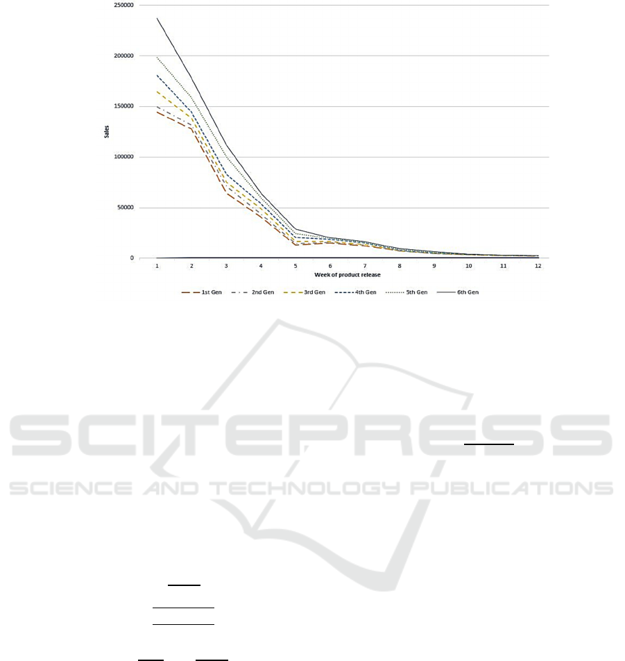
Figure 1: Historical weekly sales data for past mobile phone generation.

We visualize the historical demand data, as shown

in Figure 1 which illustrates historical data from the

past 6 years mobile phone generation. Obviously,

sales will be the most in the first week of product

release, after which there will be a significant

decrease in sales from weeks 1-6. From week six

onwards, sales fell in steady volumes to the lowest

sales in week twelve.

Then, we divide the training data set to be demand

data from year 1(first gen) to year 5 (fifth gen). For

the testing data set we use the demand data for year 6

(sixth gen). We measure the accuracy of the

forecasting method by using MAD, RMSE, and

MAPE evaluation as following equations.

𝑀𝐴𝐷 

∑













(1)

𝑅𝑀𝑆𝐸 



∑



















(2)

𝑀𝐴𝑃𝐸 

%



∑

















(3)

Noted that, to determine appropriate parameters

for each forecasting model, we implemented Time

series package in R software.

The next step after obtaining the suitable

forecasting. According to the case study company's

problem survey, we found that there is still a lack of

placement to link among inventory quantities,

demand forecasts, and production rates, whether

finished goods (FG.) or work in process (WIP.).

Therefore, it is necessary to establish this link to

manage inventory efficiently. We summarize the

linking steps as follows.

Step: 1 Calculate the number of weeks to stock

FG. and WIP. for peak demand using equation (4).

Step 2: Make production planning of FG. and

WIP. in accordance with demand and inventory

levels, as shown in Table 5.

𝑛

∑











/

(4)

where n = number of weeks required to stock FG.

and WIP.

𝐹

𝑤

= The forecast amount of demand that

exceeds capacity.

w = weeks in which the forecast demand

exceeds capacity.

k = number of weeks where demand exceeds

capacity.

Lastly, we conduct costs comparison between

proposed scenario versus that of problem scenario

based on two costs components as approximated loss

sales and inventory carrying costs.

5 RESULTS

As previously mentioned, we preliminary select

forecasting methods that are suitable for this problem.

These are (1) Holt-Winters' Seasonal Method (HW.),

(2) Autoregressive Integrated Moving Average

(ARIMA), (3) Exponential Smoothing (ETS.), and

(4) Artificial Neural Network (ANN.).

A New Product’s Demand Forecasting Using Artiﬁcial Neural Network

421

For various forecasting methods, it is necessary to

identify appropriate parameters to make the most

accurate forecasts. We summarize these parameters

for each forecast method as follows.

• HW forecasting showed that the optimal

parameters with the least forecast error were

multiplicative, with smoothing coefficients

of α = 0.0463, β=0.0443, and γ=0.8344.

• For ARIMA models, the appropriate

parameters that cause the least tolerances

are: ARIMA (0,0,1) (1,1,1) [12] with drift.

• The Exponential Smoothing (ETS) forecast

method found that optimal parameters were

α = 0.0242, β=0.0242, and γ=0.9758.

• The last method, the Neural Network (ANN)

method, found that the ideal model was

NNAR (2,1,2) [12] that was seasonal, and

lagged 1, 2, and 12 (y

t−1

.,,y

t−2

.,,y

t−12

.) of each

season were inputs, with 2 Neurons in the

Hidden Layer.

Table 3: Forecast errors for training dataset (gen1-gen5).

Metho

HW. ARIMA ETS. ANN.

MAD

1,202.20

1,280.54

1,210.91 949.97

RMSE

2,147.60

2,180.47

2,354.12 1427.46

MAPE

4.89

7.84

2.99 5.41

As shown in Table 3, ANN. method provides the

smallest forecast errors for MAD. and RMSE. cases,

while ETS. provides the smallest error in MAPE. As

mentioned in (Vandeput, 2021), selecting the suitable

demand forecast method based on using MAPE., the

forecast value is often lower than it should be. While

using RMSE., the forecast value is about the average

value. On the other hand, MAD. often gives higher

forecast value than it should be. Therefore, in this

research, we prefer average forecast value, so RMSE.

seems appropriate. Therefore, we select the right

forecasting method based on RMSE., where the best

forecast method in this case is ANN.

For testing data set, by using the ANN method, we

forecast demand of sixth generation mobile phone

and compare it with the original forecast method, see

Table 4 for the ANN. forecast results. From that table,

it shows that forecast values obtained by ANN

method are more accurate than those of the original

forecast. The original method has forecast error based

on calculated MAD, RMSE, and MAPE as 7972.17,

12410.48, and 16.46, respectively. While proposing

ANN has MAD = 3030.044, RMSE = 6046.08, and

MAPE = 5.41, respectively. In other words, ANN is

51.28% more accurate than the original forecast

method based on RMSE.

Table 4: Forecast results comparison for gen sixth model.

Week Demand Old Forecast New Forecast

(ANN.)

237,450

210,000

219,496

177,440

150,000

174,983

112,116

100,000

122,044

63,883

75,000

67,042

28,614

26,000

28,560

20,573

15,000

21,117

16,408

11,000

15,413

9,550

8,500

8,988

6,561

5,000

6,431

4,159

3,500

4,325

3,108

2,600

3,322

2,770

2,600

2,968

Then, we calculate number of weeks to stock FG.

and WIP. using equation (4). WIP. should start at

week thirty-seven while FG. should start at week

forty-two, respectively. Additionally, the capacity

should increase from 42,000 to 50,000 units. The

proposed production planning for solution scenario of

sixth generation mobile phone is conducted and

shown in Table 5.

6 SUMMARY AND DISCUSSION

In this paper, we found the major problem which is

inaccurate demand forecast that causes mis planning

of both FG. and WIP inventory volumes. Therefore,

we present the better forecast method based on ANN,

which gives 51.28% more accurate than that of the

original method. Then, we develop the proposed

solution plan that links together inventory quantities,

demand forecasts, and production rates, for both

finished goods and work in process.

We then compare the proposed solution scenario

with the problem scenario based on two cost

components as approximated loss sales and inventory

carrying costs. By knowing the sales margin, in this

case $155.00, we calculate the total sales loss value

of the problem scenario as $3,085,070.00, where the

proposed solution scenario has zero loss sales cost (no

backlog).

For the inventory carrying cost based on weekly

carrying cost for WIP inventory/unit =$0.53, and

weekly carrying cost for FG inventory/unit = $1.20,

we calculate inventory carrying cost for problem

scenario as $1,969,441.60 and that of solution

ICEIS 2024 - 26th International Conference on Enterprise Information Systems

422

Table 5: Production planning for solution scenario of sixth

generation mobile phone.

Events Week Pr.

Quantity

(FG.)

Stocks

(FG.)

Pr.

Quantity

(WIP.)

Stocks

(WIP.)

Start

WIP.

37 0 0 37,500

37,500

38 0 0 37,500

75,000

39 0 0 37,500

112,500

40 0 0 37,500

150,000

Start FG.

41 0 0 37,500

187,500

42 50,000 50,000 37,500

175,000

43 50,000 100,000 37,500

162,500

44 50,000 150,000 37,500

150,000

45 50,000 200,000 37,500 137,500

46 50,000 250,000 37,500 125,000

47 50,000 300,000 37,500 112,500

48 50,000 350,000 37,500 100,000

49 50,000 400,000 37,500 87,500

Release

FG.

50 50,000 215,000 37,500 75,000

51 50,000 90,000 37,500 62,500

52 50,000 30,000 37,500 50,000

1 50,000 18,000 37,500 37,500

2 27,061 18,061 0 10,439

3 10,439 9,500 18,944 18,944

4 14,974 9,474 0 3,970

5 3,970 4,944 8,237 8,237

6 5,409 4,853 0 2,828

7 2,828 4,181 3,423 3,423

8 2,355 4,086 0 1,068

9 1,068 2,604 2,462 2,462

scenario as $3,653,885.23. Therefore, summing loss

sales and carrying costs together we obtain the total

cost for problem and solution scenario as

$5,054,512.03 and $3,653,885.23, respectively. On

the other hand, upon implementing solution scenario,

we can reduce costs by $1,400,626.80 or by 27.71%.

Somehow, in this research, we propose the

solution scenario on forecasting only product demand

without considering other important variables such as

promotion and competitors. Therefore, for future

research, it would be more practical if we included

these variables into building the forecast model.

REFERENCES

Aburto, L., Weber, R. (2007). A sequential hybrid

forecasting system for demand prediction. In: Perner, P.

(ed.) MLDM 2007. LNCS (LNAI), vol. 4571, pp. 518–

532. Springer, Heidel-berg.

Binesh, F., Belarmino, A. M., Van der Rest, J. P., Singh, A.

K., & Raab, C. (2024). Forecasting hotel room prices

when entering turbulent times: a game-theoretic

artificial neural network model. International Journal of

Contemporary Hospitality Management, 36(4), 1044-

1065.

Fischera, T., Kraussb, C. (2017). Deep learning with long

short-term memory networks for financial market

predictions. FAU Discussion Papers in Economics.

Ghosh, S. (2020). Forecasting of demand using ARIMA

model. American Journal of Applied Mathematics and

Computing, 1(2), 11-18.

Huber, J., Gossmann, A., & Stuckenschmidt, H. (2017).

Cluster-based hierarchical demand forecasting for

perishable goods. Expert systems with applications, 76,

140-151.

Ingle, C., Bakliwal, D., Jain, J., Singh, P., Kale P., and

Chhajed, V. (2021). Demand Forecasting: Literature

Review on Various Methodologies, 12th International

Conference on Computing Communication and

Networking Technologies (ICCCNT), Kharagpur,

India, pp. 1-7, doi: 10.1109/ICCCNT51525.2021.958

0139.

Kimes, S. E., Chase, R. B., Choi, S., Lee, P. Y., & Ngonzi,

E. N. (1998). Restaurant revenue management:

Applying yield management to the restaurant industry.

Cornell Hotel and Restaurant Administration Quarterly,

39(3), 32-39.

Luckyn, B. J., Alabere, I., & Ogra, O. (2024). Predictive

Modelling for Diaper Sales in Retail: An Artificial

Neural Network Approach. Iconic Research and

Engineering Journals, 7(8).

Ma, S., Fildes, R., & Huang, T. (2016). Demand forecasting

with high dimensional data: The case of SKU retail

sales forecasting with intra-and inter-category

promotional information. Euro-pean Journal of

Operational Research, 249(1), 245-257.

Nuanmeesri, S., Poomhiran, L., Chopvitayakun, S., &

Kadmateekarun, P. (2022). Improving dropout

forecasting during the COVID-19

pandemic through

feature selection and multilayer perceptron neural

network. International Journal of Information and

Education Technology, 12(9), 851-857.

Priyadarshi, R., Panigrahi, A., Routroy, S., & Garg, G. K.

(2019). Demand forecasting at retail stage for selected

vegetables: a performance analysis. Journal of

Modelling in Management, 14(4), 1042-1063.

Ramya, B. S. S., & Vedavathi, K. (2020). An advanced

sales forecasting using machine learning algorithm.

International Journal of Innovative Science and

Research Technology, 5(5), 342-345.

Raza, K. (2017). Prediction of stock market performance by

using machine learning techniques. In: International

A New Product’s Demand Forecasting Using Artiﬁcial Neural Network

423

Conference on Innovations in Electrical Engineering

and Computational Technologies (ICIEECT), pp. 1.

Reynolds, D., Rahman, I., & Balinbin, W. (2013).

Econometric modelling of the US restaurant industry.

International Journal of Hospitality Management, 34,

317-323.

Rumbe, G., Hamasha, M., & Al Mashaqbeh, S. (2024). A

comparison of Holts-Winter and Artificial Neural

Network approach in forecasting: A case study for tent

manufacturing industry. Results in Engineering, 21,

101899.

Silva, J. C., Figueiredo, M. C., & Braga, A. C. (2019).

Econometric Demand forecasting: A case study in the

food industry. In Computational Science and Its

Applications–ICCSA 2019: 19th International

Conference, Saint Petersburg, Russia, July 1–4, 2019,

Proceedings, Part III 19 (pp. 50-63). Springer

International Publishing.

Sinthukhammoon, K., Hiranphaet, A., Sooksai, T.,

Chumkad, K., & Sonong, S. (2023, March). Demand

forecasting of Okra: case study of Okra planting

community enterprise of Kamphaeng Sean district:

International Academic Multidisciplinary Research

Conference, (pp. 198-202).

Vandeput, N. (2021). Data Science for Supply Chain

Forecasting, Berlin, Boston: De Gruyter.

https://doi.org/10.1515/9783110671124.

Xiong, R., Nichols, E. P., & Shen, Y. (2015). Deep learning

stock volatility with google domestic trends. arXiv

preprint arXiv:1512.04916.

ICEIS 2024 - 26th International Conference on Enterprise Information Systems

424