Using V2X-Information for Trajectory Prediction at Urban Intersections
Michael Kl
¨
oppel-Gersdorf
a
and Thomas Otto
Fraunhofer IVI, Fraunhofer Institute for Transportation and Infrastructure Systems, Dresden, Germany
Keywords:
Vehicle-to-Everything Communication, ITS-G5, Automated Driving, Intersections, Trajectory Prediction.
Abstract:
Crossing an urban intersection is one of the major challenges in automated/autonomous driving. This is
due to a manifold of possible interactions with other traffic participants. In this paper, we propose a tra-
jectory prediction service based on historical V2X-information gathered from Cooperative Awareness Mes-
sages (CAMs)/Basic Safety Messages (BSMs). The service allows connected vehicles to more easily navigate
the intersection by identifying possibly critical encounters, especially with traffic participants which are not
covered by the vehicle’s sensors. In comparison with approaches relying on video or other sensor data sources,
this has the advantage that Road-Side Units (RSUs), which are used for Vehicle-to-Everything (V2X) commu-
nication, are more and more available at public intersections, e.g., due to equipment rollouts all over Europe
in projects like C-Roads. The prediction service introduced in this paper is a first step in ongoing research
and will act as a baseline for further projects, where additional sensors and also more involved prediction
algorithms, e.g., based on neural networks, will be considered.
1 INTRODUCTION
Urban intersections are a hot spot for traffic acci-
dents. In Germany, in 2021, more than 20% of ac-
cidents in urban area occurred at intersections (Statis-
tisches Bundesamt (Destatis), 2022). This clearly im-
plies that navigating an urban intersection is a non-
trivial task for human drivers and even more so for au-
tomated/autonomous vehicles, compare for example
(Cosgun et al., 2017; Hubmann et al., 2018). One ma-
jor problem is the uncertainty about the other drivers’
behavior. In (Hubmann et al., 2018), four key sources
of uncertain future behavior are defined: unknown in-
tention, longitudinal uncertainty, probabilistic inter-
action and sensor uncertainty.
In this work, we want to tackle the problem of
determining the drivers’ intention based on historical
data obtained at an intersection. Here, the data is ob-
tained via V2X communication, i.e., based on either
CAM (ETSI EN 302 637-2 V1.4.1 (2019-04), 2019)
or BSM. The drivers’ intention is then determined
by calculating a most likely trajectory given the past
and current position of the vehicles under examina-
tion. The work is done in two parts, first clustering
the historical data mainly following the approach in
(Banerjee et al., 2020) and then predicting trajecto-
ries, mainly following (Wu et al., 2021). The main
a
https://orcid.org/0000-0001-9382-3062
contributions of this paper are:
• presenting a real-time capable prediction service
for connected vehicles based on V2X communi-
cation,
• using specialized distance measures between (par-
tial) trajectories to speed up computation,
• and returning several reasonable trajectories if
likely.
The remainder of the paper is organized as follows.
The methodology will be introduced in Section 2,
whereas results from a real world intersection will be
presented in Section 3. The paper is concluded in the
last section.
2 METHODOLOGY
In this section, the methodology used for clustering
and prediction is described. As the discussion is
mainly centered about the notion of (partial) trajec-
tories, we start with introducing the notion of a tra-
jectory. In general, a trajectory is considered to be
a sequence of two dimensional coordinates at certain
time steps, i.e,
T
t
n
t
0
= (⃗x(t
0
),...,⃗x(t
n
)),t
0
< t
1
< . . . < t
n
. (1)
As we are only interested in the drivers intention, not
in the dynamical behavior, the timing information is
Klöppel-Gersdorf, M. and Otto, T.
Using V2X-Information for Trajectory Prediction at Urban Intersections.
DOI: 10.5220/0012735600003702
Paper published under CC license (CC BY-NC-ND 4.0)
In Proceedings of the 10th International Conference on Vehicle Technology and Intelligent Transport Systems (VEHITS 2024), pages 473-479
ISBN: 978-989-758-703-0; ISSN: 2184-495X
Proceedings Copyright © 2024 by SCITEPRESS – Science and Technology Publications, Lda.
473

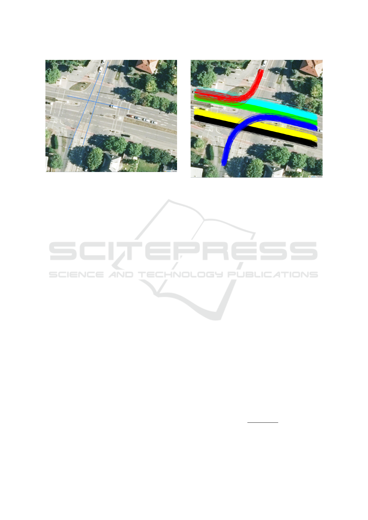
Figure 1: Overview over our reference intersection, the
Fraunhofer Smart Intersection (Kl
¨
oppel-Gersdorf et al.,
2021), located in the city of Dresden, Germany. Shown are
the principal movement vectors in approx. east-west and
north-south directions. Due to the layout of the intersec-
tion, two principal vectors are required in north-south di-
rection to successfully cluster the trajectories.
dropped. For the remainder of the paper, a trajectory
will, therefore, be considered to be a sequence of two-
dimensional coordinates, i.e,
T = (⃗x
0
,... ,⃗x
n
). (2)
2.1 Data Acquisition
V2X information in form of the CAM is used to de-
rive trajectories and we rely on information transmit-
ted by commercial vehicles. The CAMs are received
by a RSU installed at the Fraunhofer Smart Inter-
section, located in Dresden (Kl
¨
oppel-Gersdorf et al.,
2021). At the time of writing, about 0.5% of all ve-
hicles at the reference intersection use V2X technol-
ogy based on ETSI ITS-G5. While the CAM consists
of a multitude of information (e.g. dynamic informa-
tion regarding velocity and acceleration, but also the
status of turn indicators), only the current position in
WGS84 coordinates and the station id is used in this
work. Besides the position, also bounds on the posi-
tion accuracy are transmitted. The connected vehicles
on the road today typically report a position error of
approx. 3 m.
One specialty of the station id is that it changes ev-
ery 60 seconds for privacy reasons. While it would be
possible to stitch together trajectories after a change
of id, at least at the low penetration rates present to-
day, the standard discourages from doing so. There-
fore, trajectories are discarded if a change of id occurs
within the area of the intersection.
Figure 2: Part of the historical trajectories after the second
step of the hierarchical clustering scheme. Trajectory clus-
ters are now lane specific.
The trajectories used for clustering were collected
in July and August 2023. The received trajectories
were preprocessed, i.e., only the parts of the trajecto-
ries inside a rectangular area comprising the intersec-
tion were kept and partial trajectories (e.g., due to a
change in id or repeated use of the same id) were re-
moved. The first preprocessing step removed nearly
half of the received trajectories, i.e., from 3313 ini-
tially received trajectories only 1608 vehicles actu-
ally crossed the reference intersection. Removing par-
tial trajectories further reduced the trajectory count to
1535 trajectories, which were used for the clustering
step.
As a last step, coordinates were transformed from
WGS84 to an euclidic tangent plane (orthographic
projection) centered at the mid of the intersection.
2.2 Clustering
For clustering the historical trajectories, a multi step
hierarchical clustering scheme, similar to (Banerjee
et al., 2020), is used. The first step of this scheme
consists of comparing the net movement vector of the
trajectories, defined by
⃗m(T ) =⃗x
n
−⃗x
0
(3)
to predefined principal vectors p
0
,... , p
k
, describ-
ing the straight motion over the intersection. More
clearly, the cosine given by
cos(∠(⃗m(T),⃗p
i
)) =
⟨⃗m(T),⃗p
i
⟩
∥⃗m(T)∥∥⃗p
i
∥
,i = 0, . . . , k, (4)
where ⟨·,·⟩ denotes the scalar product, is used to sepa-
rate straight movements from turns and also to derive
VEHITS 2024 - 10th International Conference on Vehicle Technology and Intelligent Transport Systems
474

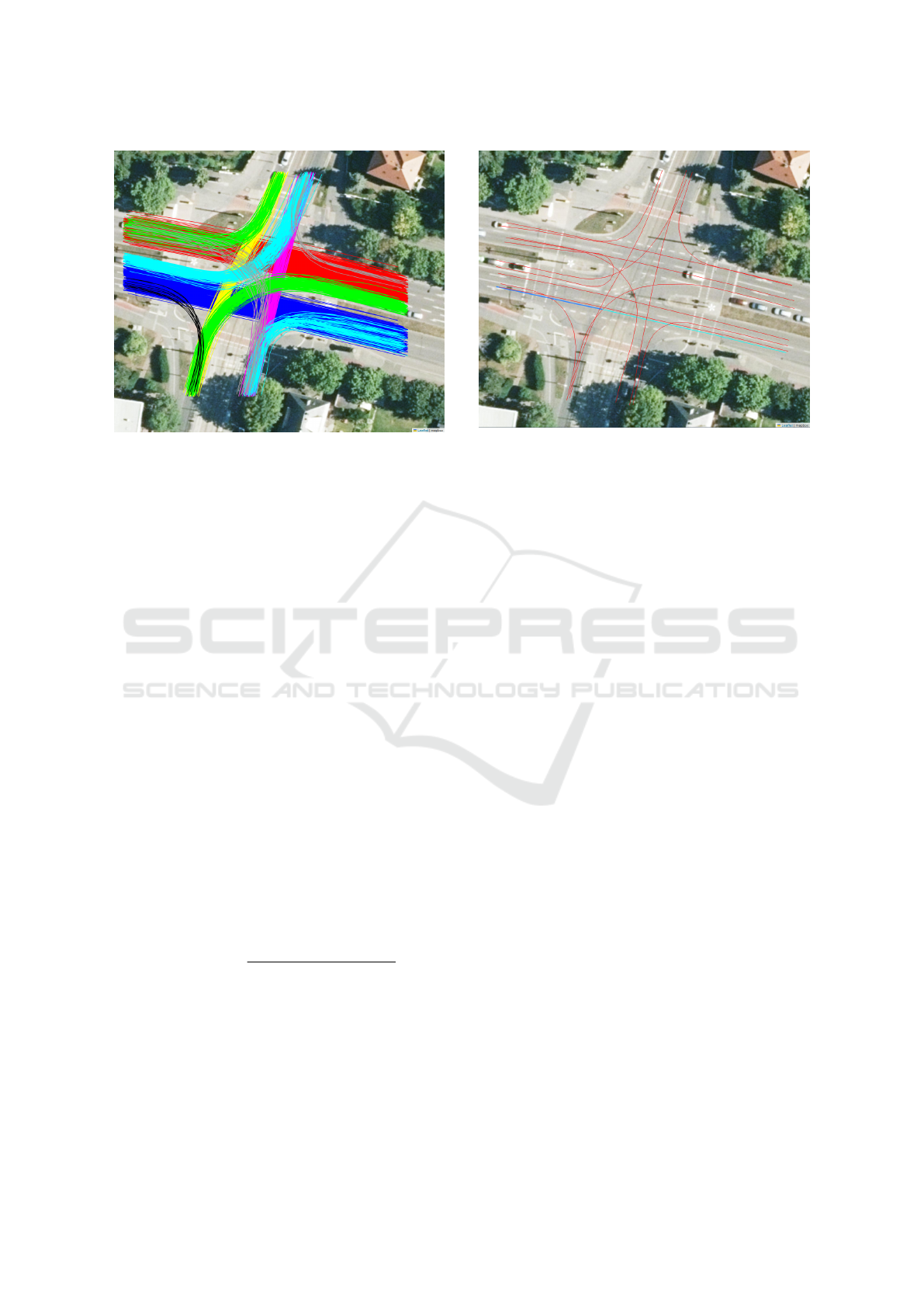
Figure 3: Historical trajectories after first step of the hier-
archical clustering scheme. Straight movements are sepa-
rated, but multi-lane traffic is still clustered into one class.
For turn movements, two relations typically clustered to-
gether. This is due to the rather simple algorithm relying on
cosine.
the general direction of motion. Due to the more com-
plicated layout of our reference intersection (tram sta-
tion between the lanes on the southern part of the in-
tersection), actually two direction vectors are required
to describe the north-south direction. The three prin-
cipal vectors of the reference intersection are shown
in Fig. 1, whereas the result of the first clustering step
is shown in Fig. 3.
In a next step, the turning movements and the
streams along the two-lane streets (east-west and
west-east direction) need to be separated. In (Baner-
jee et al., 2020) the position of the stop bar is used
to differentiate the different turning movements (e.g.,
the green trajectories in Fig. 3). Here, a slightly dif-
ferent approach based on a distance measure is pro-
posed. Let the length of a trajectory T be defined as
length(T ) =
n
∑
i=1
∥⃗x
i
−⃗x
i−1
∥. (5)
Then, similar to (Wu et al., 2021), the distance be-
tween two trajectories is defined as
dist(T
1
,T
2
) =
area(T
1
,T
2
)
length(T
1
) + length(T
2
)
, (6)
where the area(·,·) is defined by the area of the poly-
gon generated by the two trajectories, i.e., if T
1
=

⃗x
1
0
,... ,⃗x
1
n
1

and T
2
=

⃗x
2
0
,... ,⃗x
2
n
2

, the area of the
polygon

⃗x
1
0
,... ,⃗x
1
n
1
,⃗x
2
n
2
,... ,⃗x
2
0

. Note that the co-
ordinates of the second trajectory are reversed here.
This area can be computed by geometric packages
like Shapely in Python. This approach does not
Figure 4: Reference trajectories derived for all driving re-
lations in red. Also shown is one of the evaluation trajec-
tories. Dark blue shows the part of the trajectory used for
prediction, whereas the remainder of the trajectory is shown
in cyan. This part was only used for the computation of Av-
erage Displacement Error (ADE) and Final Displacement
Error (FDE).
need Dynamic Time Warping (Kruskal and Liberman,
1983) or the variant FastDTW (Salvador and Chan,
2007) used by the authors of (Banerjee et al., 2020;
Wu et al., 2021). This reduces the computation time
of the algorithm significantly, because even if Fast-
DTW is linear in time and space, it still requires a
rather long computation time.
Separating the turn movements consists of a
choosing a random reference trajectory inside the
cluster, e.g., the first one T
1
. For all trajectories in
the cluster T
1
,... , T
l
the distance to the reference tra-
jectory is computed. Trajectories following a similar
movement will show only minimal distance in com-
parison to movements on the other side of the inter-
section. Both clusters can then easily be separated us-
ing a simple threshold for distance. This computation
is linear in the number of elements in the cluster.
Separating the two-lane traffic uses a similar pro-
cedure. Again, starting with a reference trajectory T
1
,
the distances to all other trajectories in this cluster are
computed. A trajectory T
b
1
is computed as
T
b
1
= arg max
T =T
2
,...,T
l
dist(T
1
,T ). (7)
A second trajectory T
b
2
is computed as
T
b
2
= arg max
T =T
1
,...,T
l
dist(T
b
1
,T ). (8)
Figuratively speaking, T
b
1
and T
b
2
are the two out-
ermost trajectories of the cluster. As a last step, the
distance of all trajectories to T
b
1
and T
b
2
are calcu-
lated. Finally, the trajectories are clustered depending
Using V2X-Information for Trajectory Prediction at Urban Intersections
475

9
1 1 7
2 7 8
2 0 4
1 2 2
6 3
4
5 9
7 8
2 1
1 4
2 3 2
2 3 0
9 4
1 0
2
5
2 2
1 2
8
3
0
3
7
1
5
1 7
1 4
6
0
e n e s e w _ 1 e w _ 2 n s n w o t h e r s e s n s w u _ t u r n w e _ 1 w e _ 2 w n w s
0
5 0
1 0 0
1 5 0
2 0 0
2 5 0
3 0 0
C o u n t
D r i v i n g r e l a t i o n
T r a i n
E v a l u a t i o n
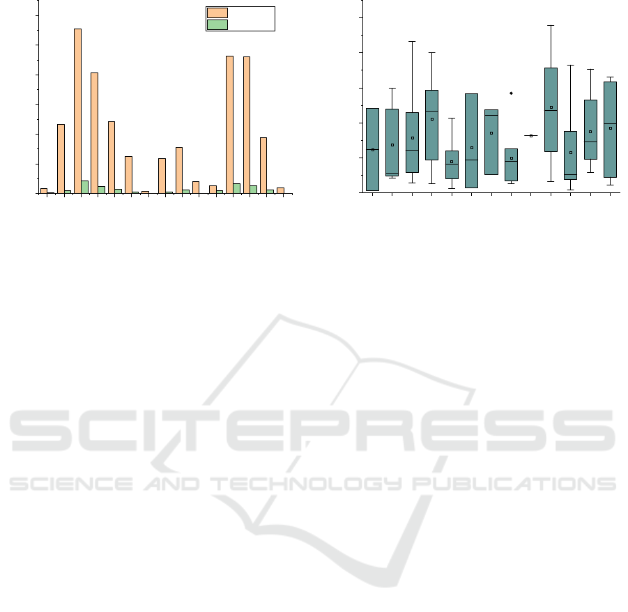
Figure 5: Distribution of the single driving movements for
training and evaluation data set. A χ
2
homogeneity test re-
vealed significant differences between the two datasets re-
garding the distribution of the single driving maneuvers.
on whether they are closer to T
b
1
or T
b
2
. This process
is also linear in the number of elements in the cluster,
even though it uses four passes over all elements.
A part of the derived clusters are shown in Fig.
2. Please note that no spectral clustering is carried
out, i.e., there is only one cluster for all movements,
e.g., in west-north direction. While this limits the
ability of the presented approach to detect outliers,
it also reduces computation time immensely, since
the computational demands of spectral clustering in-
crease quadratically with the number of elements in
the cluster.
The last step of the clustering algorithm consists
of determining reference trajectories for all clusters.
Like (Banerjee et al., 2020), a representative trajec-
tory for each cluster is computed as the central ele-
ment. The approach used is the same as in separating
the straight movements, i.e., beginning with a random
element of the cluster one outer trajectory is calcu-
lated. In a second step, the distance of all trajecto-
ries of the cluster to this outer trajectory a computed.
The representative trajectory is chosen as the trajec-
tory with the median distance. The representative tra-
jectories for all movement relations are shown in Fig.
4.
2.3 Prediction
For predicting the future movement of a given partial
trajectory (see Fig. 4 for an example), we loosely fol-
low (Wu et al., 2021) in that we use the representative
trajectories, derived above, to first calculate possible
movement candidates. Instead of using a neural net-
work, as done in the previous mentioned work, we
decided to compare the partial trajectories directly to
e n e s e w _ 1 e w _ 2 n s n w s e s n s w u _ t u r n w e _ 1 w e _ 2 w n
0
1 0
2 0
3 0
4 0
5 0
D r i v i n g r e l a t i o n
P a r t i a l t r a j e c t o r y l e n g t h [ m ]
Figure 6: Box plot showing the distribution of the length of
the partial trajectories per driving relation. These trajecto-
ries have a length of up to 50 m.
the historical data. While it may be intuitive to use
the previously defined dist(·,·) to derive the candi-
dates, this actually proved not successful in practice.
One reason for this is that some of the polygons con-
structed in distance calculation are self-intersecting,
leading to problems of computing the area (Shapely
does not guarantee correct area computation for self-
intersecting polygons). Therefore, a new distance
measure based on ADE and FDE was used. Here,
ADE(T
1
,T
2
) = n
−1
n
∑
i=0
algebraicdist(⃗x
1
i
,T
2
), (9)
FDE(T
1
,T
2
) = algebraicdist(⃗x
1
n
,T
2
), (10)
where algebraicdist(·,·)) is the algebraic distance of
the point in the first argument to the line string in the
second argument. The final distance measurement is
computed as
weighteddist(T
1
,T
2
) =
αADE(T
1
,T
2
) + (1 − α)FDE(T
1
,T
2
), (11)
for 0 ≤ α ≤ 1. The reason for giving extra weight to
the last point of the partial trajectory are trajectories as
shown in Fig. 4. While this is most certainly a straight
movement, it is still rather close to the representative
trajectory of the right turn. Giving additional weight
to the last coordinate increases this distance. Can-
didate movement relations are derived by computing
weighteddist(·,·) for the partial trajectory and all rep-
resentative trajectories. Candidates are selected, if the
distance is not larger than a given threshold.
In a second step, the partial trajectory will be com-
pared against all trajectories in the candidate clusters,
again using weighteddist. As prediction, the histor-
ical trajectory with overall the least distance is re-
turned. The information about the possible candidate
clusters is also available.
VEHITS 2024 - 10th International Conference on Vehicle Technology and Intelligent Transport Systems
476

e n e s e w _ 1 e w _ 2 n s n w s e s n s w u _ t u r n w e _ 1 w e _ 2 w n
0 . 0
0 . 2
0 . 4
0 . 6
0 . 8
D r i v i n g r e l a t i o n
A v e r g a g e D i s p l a c e m e n t E r r o r [ m ]
(a)
e n e s e w _ 1 e w _ 2 n s n w s e s n s w u _ t u r n w e _ 1 w e _ 2 w n
0 . 0 0
0 . 0 5
0 . 1 0
0 . 1 5
0 . 2 0
0 . 2 5
0 . 3 0
D r i v i n g r e l a t i o n
F i n a l D i s p l a c e m e n t E r r o r [ m ]
(b)
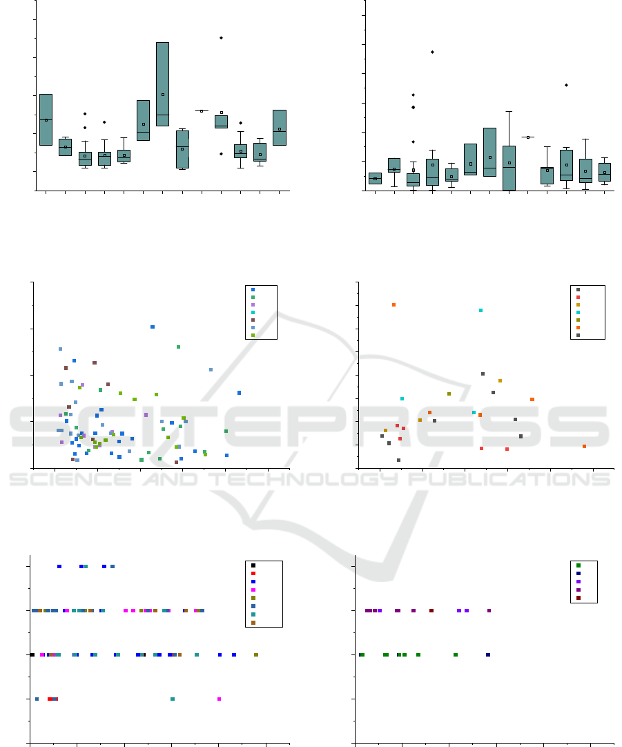
Figure 7: Average Displacement Error (ADE) (a) and Final Displacement Error (FDE) (b) per driving relation.
0 1 0 2 0 3 0 4 0 5 0
0 . 0
0 . 1
0 . 2
0 . 3
0 . 4
e w _ 1
e w _ 2
n s
s e
s n
w e _ 1
w e _ 2
A v e r a g e D i s p l a c e m e n t E r r o r [ m ]
P a r t i a l t r a j e c t o r y l e n g t h [ m ]
(a)
0 1 0 2 0 3 0 4 0 5 0
0 . 0
0 . 1
0 . 2
0 . 3
0 . 4
0 . 5
0 . 6
0 . 7
0 . 8
e n
e s
n w
s e
s w
u _ t u r n
w n
A v e r a g e D i s p l a c e m e n t E r r o r [ m ]
P a r t i a l t r a j e c t o r y l e n g t h [ m ]
(b)
Figure 8: Length of the partial trajectory vs Average Displacement Error (ADE), for straight movements (a) and turns (b).
0 1 0 2 0 3 0 4 0 5 0
0
1
2
3
4
e n
e s
e w _ 1
e w _ 2
u _ t u r n
w e _ 1
w e _ 2
w n
N u m b e r o f c a n d i d a t e s
P a r t i a l t r a j e c t o r y l e n g t h [ m ]
(a)
0 1 0 2 0 3 0 4 0 5 0
0
1
2
3
4
n s
n w
s e
s n
s w
N u m b e r o f c a n d i d a t e s
P a r t i a l t r a j e c t o r y l e n g t h [ m ]
(b)
Figure 9: Length of the partial trajectory vs. the number of potential representative trajectories, for vehicles entering the
intersection from east or west (a) and north or south (b). These figures also show that we were able to generate candidate
trajectories for every trajectory in the evaluation set.
Using V2X-Information for Trajectory Prediction at Urban Intersections
477

2.4 Implementation
The RSU saves the position and station id of the re-
ceived CAM in a comma-separated text file. These
log files are gathered periodically from the RSU.
Analysis is then performed with Python, mainly using
GeoPandas
1
and Shapely
2
. The orthographic projec-
tion is handled by PyProj
3
. Visualizations are gener-
ated using Folium
4
. Clustering the 1535 historical tra-
jectories takes about four seconds, predicting the 105
partial trajectories takes about ten seconds, or about
0.1s for each. Please note that the time for prediction
increases if the historical database increases, but this
growth is linear in trajectory size and can easily be
handled by optimizing the code and using paralleliza-
tion.
3 RESULTS AND DISCUSSION
For the evaluation of the proposed algorithm, 105 tra-
jectories collected in February 2024 were used. An
overview over these trajectories as well as over the
training data regarding the distribution of driving re-
lation is shown in Fig. 5. These 105 trajectories
were randomly shortened to arrive at partial trajecto-
ries (comp. Fig. 4). An overview over the length of
the partial trajectories with regard to driving relation
are shown in Fig. 6.
For all of the 105 partial trajectories a prediction
(one single trajectory) was computed. The Average
Displacement Error (ADE) and Final Displacement
Error (FDE) of these predictions against the actually
driven trajectories is shown in Fig. 7. ADE for the
straight movements (ew, ew, ns, sn) is usually smaller
than for the turning movements. This is rather intu-
itive, since first there are much more historical tra-
jectories for the straight movements (comp. Fig. 5)
and there is also much more variability in a turning
movement in comparison to a straight movement. On
the other hand, final displacement error shows a rather
uniform distribution. This is also clear, since the
movement ends at the egress lane and does not leave
much room for deviation. The values for ADE and
FDE reported here are in line with the values reported
in (Wu et al., 2021), maximum ADE is less than 0.8m
and maximum FDE is even less than 0.25m.
In a further analysis step, ADE vs. length of
the partial trajectory was examined. Intuitively, one
would expect ADE to decrease with increasing length
1
https://geopandas.org/en/stable/
2
https://pypi.org/project/shapely/
3
https://pypi.org/project/pyproj/
4
https://python-visualization.github.io/folium/latest/
of the partial trajectory. Looking at Fig. 8 certainly
shows a trend, but this is much less pronounced than
one might expect. For straight movements, Pearson’s
correlation coefficient is about −0.1, whereas it is
−0.02 for turning movements. The disparity in avail-
able historical data could be one explanation for this
effect.
In a last step, the numbers of candidates derived in
the first step of the prediction algorithm vs. the length
of the trajectory was analyzed. Again, one would sus-
pect fewer candidates the longer the trajectory. As
shown by Fig. 9, this is certainly true for movements
entering the intersection from east or west along the
two-lane streets. Still, two possible candidates are
calculated most of the time. This is attributed to the
inaccuracy in the initial data, which nearly equals the
width of a lane, making it difficult to determine the
lane the vehicle actually used in the past. On the other
hand, vehicles entering from the north always get two
candidates assigned (which is the maximum number
of possible driving directions, a left turn is disallowed
at this entrance to the intersection), whereas vehicles
entering from the south always get assigned three can-
didates (also the maximum). This is attributed to the
length of the partial trajectory, even at about 30m into
the intersection no driving relation can be ruled out.
4 CONCLUSIONS AND FUTURE
WORK
In this paper, a simple and fast method to predict ve-
hicle movement, based on historical V2X data, is pro-
posed. Although no modern neural networks, like
Long-Short-Term Memorys (LSTMs), are used, the
results are comparable, especially for driving rela-
tions with sufficient historical data. As mentioned be-
fore, this is just a first step in an ongoing research
effort and will act as a base line for further research.
In the current work, only the movement of vehi-
cles is predicted. Especially at urban intersections,
Vulnerable Road User (VRU) might have an influence
on the motion of automated/autonomous vehicles. At
the moment, there is no V2X message to track these
traffic participants directly, although ETSI recently
specified the VRU Awareness Message (VAM). There
is also the chance of indirect detection through the
use of Collective Perception Message (CPM), which
allows vehicles and infrastructure to publish their sen-
sor readings. Nonetheless, predicting VRUs also
needs new approaches, as their possibility of move-
ment is much more unconstrained than vehicular mo-
tion. Some possible methods for predicting pedes-
trian movement are already benchmarked in (Uhle-
VEHITS 2024 - 10th International Conference on Vehicle Technology and Intelligent Transport Systems
478

mann et al., 2023).
ACKNOWLEDGEMENTS
This research is financially supported by the Ger-
man Federal Ministry for Economic Affairs and Cli-
mate Action (BMWK) under grant number FKZ
19A22009F (VALISENS). We would like to thank
Hsi Chen for carrying out some of the analysis steps.
REFERENCES
Banerjee, T., Huang, X., Chen, K., Rangarajan, A., and
Ranka, S. (2020). Clustering object trajectories for
intersection traffic analysis [clustering object trajecto-
ries for intersection traffic analysis]. Proceedings of
the 6th International Conference on Vehicle Technol-
ogy and Intelligent Transport Systems - VEHITS.
Cosgun, A., Ma, L., Chiu, J., Huang, J., Demir, M., A
˜
non,
A. M., Lian, T., Tafish, H., and Al-Stouhi, S. (2017).
Towards full automated drive in urban environments:
A demonstration in gomentum station, california. In
2017 IEEE Intelligent Vehicles Symposium (IV), pages
1811–1818.
ETSI EN 302 637-2 V1.4.1 (2019-04) (2019). ETSI EN
302 637-2 V1.4.1 (2019-04) Intelligent Transport Sys-
tems (ITS); Vehicular Communications; Basic Set of
Applications; Part 2: Specification of Cooperative
Awareness Basic Service. Standard, ETSI.
Hubmann, C., Schulz, J., Becker, M., Althoff, D., and
Stiller, C. (2018). Automated driving in uncertain en-
vironments: Planning with interaction and uncertain
maneuver prediction. IEEE Transactions on Intelli-
gent Vehicles, 3(1):5–17.
Kl
¨
oppel-Gersdorf, M., Trauzettel, F., Koslowski, K., Pe-
ter, M., and Otto, T. (2021). The fraunhofer ccit
smart intersection. In 2021 IEEE International In-
telligent Transportation Systems Conference (ITSC),
pages 1797–1802. IEEE.
Kruskal, J. and Liberman, M. (1983). The symmetric time-
warping problem: From continuous to discrete. Time
Warps, String Edits, and Macromolecules: The The-
ory and Practice of Sequence Comparison.
Salvador, S. and Chan, P. (2007). Toward accurate dynamic
time warping in linear time and space. Intell. Data
Anal., 11(5):561–580.
Statistisches Bundesamt (Destatis), . (2022). Verkehr
Verkehrsunf
¨
alle 2021. Statistisches Bundesamt
(Destatis), 2022.
Uhlemann, N., Fent, F., and Lienkamp, M. (2023). Evaluat-
ing Pedestrian Trajectory Prediction Methods for the
Application in Autonomous Driving. arXiv e-prints,
page arXiv:2308.05194.
Wu, A., Banerjee, T., Rangarajan, A., and Ranka, S. (2021).
Trajectory prediction via learning motion cluster pat-
terns in curvilinear coordinates. In 2021 IEEE Inter-
national Intelligent Transportation Systems Confer-
ence (ITSC), pages 2200–2207.
Using V2X-Information for Trajectory Prediction at Urban Intersections
479