Efficient Real-Time Obstacle Avoidance Using Multi-Objective Nonlinear
Model Predictive Control and Semi-Smooth Newton Method
Mostafa Emam
a
, Thomas Rottmann and Matthias Gerdts
b
Department of Aerospace Engineering, Institute of Applied Mathematics and Scientific Computing, University of the
Bundeswehr Munich, 85579, Neubiberg, Germany
Keywords:
Automated Driving, Obstacle Avoidance, Path Planning, Mutli-Objective NMPC, Semi-Smooth Newton
Method.
Abstract:
This work discusses the theory and methodology of applying Nonlinear Model Predictive Control (NMPC) in
an efficient manner to achieve real-time path planning and obstacle avoidance for autonomous vehicles. First,
we explain the optimization problem formulation and the numerical solution approach using a semi-smooth
Newton method adapted for nonlinear problems. Then, an MPC path planning problem is described in terms of
the vehicle model, the controller design, and the mathematical representation of obstacles as proper system
constraints. Afterwards, the developed controller is numerically evaluated for different vehicle models in
a simulated environment to dynamically assess its flexibility and real-time performance, which serves as a
prerequisite to deferred real-life testing.
1 INTRODUCTION
Optimal Control has evolved as the natural successor
to the Calculus of Variations to address optimization
problems with path (state/control) constraints, contrary
to the classic unconstrained problems proposed by
early mathematicians and philosophers (Sussmann and
Willems, 1997). The incorporation of these inequality
constraints added another layer of complexity that was
first solved in the late 1950s with the introduction of
Pontryagin’s Maximum Principle (PMP), yet the devel-
oped methodologies can be traced back to the work of
earlier renowned mathematicians like Euler, Lagrange,
and Legendre (Chachuat, 2007). A particular approach
to handle constrained optimization problems is Model
Predictive Control (MPC), also known as Receding
Horizon Control (RHC), which was initially developed
to tackle problems in the oil and gas industry in the
1980s (Morari and H. Lee, 1999), but has progressed
since then to represent an effective and flexible frame-
work that can be employed to optimally solve multi-
variable Optimal Control Problems (OCPs) with mixed
state-control constraints (Gr
¨
une and Pannek, 2011).
Owing to its versatility, MPC has gained a notice-
able popularity in autonomous driving applications,
a
https://orcid.org/0000-0003-4942-1183
b
https://orcid.org/0000-0001-8674-5764
especially in path planning, trajectory following and
multi-objective vehicle control (Vu et al., 2021; Qin
et al., 2023; Musa et al., 2021; Emam and Gerdts,
2022). However, MPC comes with the caveat that
the determined solution is only optimal for the exact
problem parameters, e.g., the initial states, thus model
deviations and system uncertainties will quickly inval-
idate the solution optimality. In other words, only a
subset of the calculated control trajectory u
∗
can be
applied before the need arises to re-solve the OCP
to yield an optimal u
∗
(Rawlings and Mayne, 2009).
In traditional MPC, only the first control sequence
is applied and the OCP is re-solved every time step,
which represents a computational bottleneck for real-
time applications and is the main drive for research
effort towards efficient solution techniques (Diehl
et al., 2005).
In this work, we tackle the MPC real-time restric-
tion by adapting a previously implemented efficient
semi-smooth Newton method, originally designed for
linear systems (Emam and Gerdts, 2023), so that it
handles nonlinear Discrete Optimal Control Problems
(DOCPs). We validate our approach by developing a
generic controller with mixed state-control constraints
for autonomous path planning, and propose a math-
ematically efficient method to incorporate obstacle
avoidance using smooth, continuously differentiable
envelopes, which enables faster convergence of the
178
Emam, M., Rottmann, T. and Gerdts, M.
Efficient Real-Time Obstacle Avoidance Using Multi-Objective Nonlinear Model Predictive Control and Semi-Smooth Newton Method.
DOI: 10.5220/0012738400003702
Paper published under CC license (CC BY-NC-ND 4.0)
In Proceedings of the 10th International Conference on Vehicle Technology and Intelligent Transport Systems (VEHITS 2024), pages 178-189
ISBN: 978-989-758-703-0; ISSN: 2184-495X
Proceedings Copyright © 2024 by SCITEPRESS – Science and Technology Publications, Lda.

problem solution. The controller is implemented as
part of an integrated virtual testing environment and
is evaluated for different vehicle models to ensure its
flexibility and effectiveness. Thorough explanation
and numerical results are discussed in the sequel.
2 CONTROL PROBLEM AND
NUMERICAL SOLUTION
The basic MPC scheme entails solving instances of
a parametric DOCP with specific objectives, system
dynamics, and path constraints and, provided that a
solution exists, employs this solution to derive the
optimal feedback control law (Morari and H. Lee,
1999). This incorporates some implicit assumptions,
e.g., the instantaneous computation of the DOCP’s
numerical solution and the absence of delays when
applying the control inputs (Gr
¨
une and Pannek, 2011).
Since this does not adequately reflect real applications,
some adaptations are required before implementing
the MPC approach, such as prediction, re-optimization,
and sensitivity updates. For a comprehensive overview
on formulating, discretizing, and solving OCPs, the
reader is directed to (Gerdts, 2023), and for specific
MPC considerations to (Palma, 2015). With brevity
in mind, we focus in this section on the basic MPC
scheme and begin discussing the strategy for calcu-
lating the numerical solution of the DOCP.
2.1 Newton Method for DOCPs
Newton’s algorithm is a fundamental approach to reach
an existing solution z
∗
∈ R
n
z
that satisfies the nonlinear
and continuously differentiable function φ(z) = 0 with
φ : R
n
z
→ R
n
z
. It starts with an initial estimate ˜z and
if φ(˜z) ̸= 0 , computes a direction d to update ˜z using a
linear approximation of φ around ˜z from the first two
terms in its Taylor series expansion. d is the solution
of the linear system:
∇φ(˜z
(ℓ)
)d
(ℓ)
= −φ(˜z
(ℓ)
),
˜z
(ℓ+1)
= ˜z
(ℓ)
+ d
(ℓ)
, ℓ = 0, 1,2,...
(1)
where ∇φ(˜z) is the Jacobian of φ around ˜z , ˜z
(ℓ+1)
is
the new estimate, and ℓ is the iteration index. Provided
that ∇φ(˜z
(ℓ)
) is nonsingular, the process repeats and
iteratively approaches φ(˜z
(ℓ)
) ≈ 0 , such that ˜z
(ℓ)
≈ z
∗
(within a specified error margin) (Chachuat, 2007;
Gerdts, 2023). To employ this method, we first need to
formulate the DOCP with its system dynamics, objec-
tive function, constraints, and boundary conditions, as
a differentiable function, which we will now discuss.
Consider the implicit structured nonlinear OCP in
discrete time k ∈ N
0
with general boundary conditions:
Minimize
J(z, p) :=
N
∑
k=0
F
0
(k, z
k
, p) (2)
w.r.t. z = (z
0
,.. .,z
N
)
⊤
∈ R
(N+1)
n
z
, p ∈ R
n
p
, and
s.t. the constraints
F(k, z
k+1
,z
k
, p) = 0, k = 0,.. .,N −1, (3)
G(k, z
k
, p) ≤ 0, k = 0,... ,N, (4)
Ψ(z
0
,z
N
, p) = 0. (5)
Herein, z
k
∈ R
n
x
×n
u
denotes the state and control
vector at time k ∈ N
0
, p ∈ R
n
x
is the initial state vector.
(3) represents the nonlinear system dynamics, (4) are
the mixed state and control constraints, and (5) denote
the general boundary conditions. Linearization of the
constraints at some ˆz and ˆp yields:
G
k
z
k+1
+ F
k
z
k
+ P
k
p = −F[k], k = 0,... ,N − 1, (6)
E
k
z
k
+ D
k
p ≤ −G[k], k = 0,...,N, (7)
Ψ
0
z
0
+ Ψ
N
z
N
+ P
N
p = −Ψ( ˆz
0
, ˆz
N
, ˆp) (8)
where F[k] indicates the evaluation of F at k, ˆz, ˆp
and likewise for other occurrences. Alternatively, the
problem can be formulated with separated boundary
conditions using:
Ψ(z
0
,z
N
, p) =

Ψ
0
(z
0
, p)
Ψ
N
(z
N
, p)

= 0 (9)
and linearization at ˆz and ˆp yields:

Ψ
0
0

z
0
+

0
Ψ
N

z
N
+

P
0
P
N

p =
−

Ψ
0
( ˆz
0
, ˆp)
Ψ
N
( ˆz
N
, ˆp)

(10)
Herein
G
k
= F
′
z
k+1
[k], F
k
= F
′
z
k
[k], P
k
= F
′
p
[k],
E
k
= G
′
z
[k], D
k
= G
′
p
[k],
Ψ
0
= Ψ
′
z
0
( ˆz
0
, ˆz
N
, ˆp), Ψ
N
= Ψ
′
z
N
( ˆz
0
, ˆz
N
, ˆp),
P
N
= Ψ
′
p
( ˆz
0
, ˆz
N
, ˆp)
and respectively for separated boundary conditions:
Ψ
0
= Ψ
′
0,z
( ˆz
0
, ˆp), P
0
= Ψ
′
0,p
( ˆz
0
, ˆp)
Ψ
N
= Ψ
′
N,z
( ˆz
N
, ˆp), P
N
= Ψ
′
N,p
( ˆz
N
, ˆp)
Let λ = (λ
⊤
0
,.. .,λ
⊤
N−1
)
⊤
, µ = (µ
⊤
0
,.. .,µ
⊤
N
)
⊤
, and
σ denote the vectors of Lagrange multipliers for the
constraints (3), (4), and (5) respectively, such that
Efficient Real-Time Obstacle Avoidance Using Multi-Objective Nonlinear Model Predictive Control and Semi-Smooth Newton Method
179

σ = (σ
0
,σ
N
)
⊤
for the separated boundary conditions.
The DOCP Lagrange function is defined as:
L(z, p,λ, µ,σ) :=κ(z
0
,z
N
, p,µ
N
,σ)
+
N−1
∑
k=0
H(k,z
k+1
,z
k
, p,λ
k
,µ
k
)
(11)
with:
κ(z
0
,z
N
, p,µ
N
,σ) = F
0
(N,z
N
, p) + µ
⊤
N
G(N,z
n
, p)
+ σ
⊤
Ψ(z
0
,z
N
, p)
and the Hamilton function is defined as:
H(k,z
k+1
,z
k
, p,λ
k
,µ
k
) :=F
0
(k, z
k
, p)
+ λ
⊤
k
F(k, z
k+1
,z
k
, p)
+ µ
⊤
k
G(k, z
k
, p)
(12)
Provided that some constraint qualification is
satisfied and given a local minimum z
∗
, there exists
Lagrangian multipliers that satisfy the upcoming
first order necessary Karush-Kuhn-Tucker (KKT)
conditions (Chachuat, 2007; Gerdts and Kunkel, 2008).
These conditions can be solved by utilizing a semi-
smooth Newton method, and we highlight that they
shall be necessary and sufficient for a global minimum
of the DOCP, on condition that the matrix H
k
is
positive semi-definite and symmetric ∀k ∈ N
0
(Gerdts,
2023). The KKT conditions read:
0 = ∇
z
0
L = ∇
z
0
κ + ∇
z
k
H[0]
0 = ∇
z
k
L = ∇
z
k
H[k] + ∇
z
k+1
H[k −1]
0 = ∇
z
N
L = ∇
z
N
κ + ∇
z
k+1
H[N − 1]
0 = ∇
p
L = ∇
p
κ +
N−1
∑
k=0
∇
p
H[k]
with the second derivatives (for k = 1,...,N −1):
H
0
= ∇
2
z
0
,z
0
L = ∇
2
z
0
,z
0
κ + ∇
2
z
k
,z
k
H[0]
H
k
= ∇
2
z
k
,z
k
L = ∇
2
z
k
,z
k
H[k] + ∇
2
z
k+1
,z
k+1
H[k −1]
H
N
= ∇
2
z
N
,z
N
L = ∇
2
z
N
,z
N
κ + ∇
2
z
k+1
,z
k+1
H[N − 1]
Q = ∇
2
p,p
L = ∇
2
p,p
κ +
N−1
∑
k=0
∇
p,p
H[k]
Q
⊤
0
= ∇
2
p,z
0
L = ∇
2
p,z
0
κ + ∇
2
p,z
k
H[0]
Q
⊤
k
= ∇
2
p,z
k
L = ∇
2
p,z
k
H[k] + ∇
2
p,z
k+1
H[k −1]
Q
⊤
N
= ∇
2
p,z
N
L = ∇
2
p,z
N
κ + ∇
2
p,z
k+1
H[N − 1]
Ξ
0,N
= Ξ
⊤
N,0
= ∇
2
z
0
,z
N
L = ∇
2
z
0
,z
N
κ
J
k
= ∇
2
z
k
,z
k+1
L = ∇
2
z
k
,z
k+1
H[k]
J
⊤
k−1
= ∇
2
z
k
,z
k−1
L = ∇
2
z
k+1
,z
k
H[k −1]
To incorporate the status of inequality constraints
(active/inactive), we additionally enforce the comple-
mentarity conditions:
0 ≤ µ
k
⊥ −G(k,z
k
, p) ≥ 0, k = 0, ...,N
by utilizing the convex and Lipschitz continuous
Fischer-Burmeister function ϕ : R
2
→ R (Jiang, 1999;
Jiang and Qi, 1997) defined by (Fischer, 1992):
ϕ(a,b) :=
p
a
2
+ b
2
− a − b,
which has the appealing property that ϕ(a,b) = 0 holds
either when a,b ≥ 0 or ab = 0 (Gerdts and Kunkel,
2009). Hence, the complementarity conditions can be
equivalently reformulated as the non-smooth equation:
ϕ(−G(k,z
k
, p),µ
k
) = 0, k = 0,...,N
and since ∂ϕ does not exist at the origin, we instead
utilize Clarke’s generalized Jacobian of ϕ to determine
its value (Gerdts and Kunkel, 2008).
Combining the necessary and sufficient conditions
with the constraints produces the nonlinear equation:
F (η) = 0,
η = (σ
⊤
,z
⊤
0
,µ
⊤
0
,λ
⊤
0
,.. .,z
⊤
N−1
,µ
⊤
N−1
,λ
⊤
N−1
,z
⊤
N
,µ
⊤
N
)
⊤
(13)
with:
F (η) =




Ψ(z
0
,z
N
, p)
β
0
(η)
.
.
.
β
N
(η)




,
where for k = 0,... ,N − 1:
β
k
=



∇
z
k
L(z
(ℓ)
, p
(ℓ)
,λ
(ℓ)
,µ
(ℓ)
,σ
(ℓ)
)
ϕ(−G(k,z
(ℓ)
k
, p
(ℓ)
),µ
(ℓ)
k
)
F(k, z
(ℓ)
k+1
,z
(ℓ)
k
, p
(ℓ)
)



,
β
N
=
∇
z
N
L(z
(ℓ)
, p
(ℓ)
,λ
(ℓ)
,µ
(ℓ)
,σ
(ℓ)
)
ϕ(−G(N,z
(ℓ)
N
, p
(ℓ)
),µ
(ℓ)
N
)
!
.
Applying a semi-smooth Newton method to this
nonlinear and non-smooth equation (13) results in the
iteration:
V
ℓ
d
(ℓ)
= −F (η
(ℓ)
),
η
(ℓ+1)
= η
(ℓ)
+ d
(ℓ)
, ℓ = 0, 1,2,...
(14)
which follows (1), where V
ℓ
∈ ∂F (η
(ℓ)
) and ∂F (η
(ℓ)
)
is Clarke’s generalized Jacobian of F (Clarke, 1990).
For simplification, we assume no mixed derivatives
exist, i.e., ∇
2
z
k
,z
k+1
H[k] = ∇
2
z
k+1
,z
k
H[k] = 0, and Ξ
0,N
=
Ξ
N,0
= 0 . This presents us with the following linear
Newton system (14) that comprises a sparse, block-
banded matrix structure:
VEHITS 2024 - 10th International Conference on Vehicle Technology and Intelligent Transport Systems
180

[!th]








Ω
0
Ω
⊤
0
Γ
0
Ω
1
Ω
⊤
1
Γ
1
.
.
.
.
.
.
.
.
.
Ω
N
Ω
⊤
N
Γ
N














d
σ
d
0
d
1
.
.
.
d
N






=
−







Ψ(z
(ℓ)
0
,z
(ℓ)
N
, p
(ℓ)
)
β
0
β
1
.
.
.
β
N







that can be exploited and efficiently factorized using,
for example, the LAPACK routines for LU decompo-
sition (Britzelmeier and Gerdts, 2020). In addition, it
has been long established that structural exploitation
can significantly increase the efficiency and reliability
of solving sparse banded matrices by orders of magni-
tude (Morari and H. Lee, 1999; Gerdts, 2023).
For k = 0, ...,N − 1, we have:
d
k
= (d
⊤
z
k
,d
⊤
µ
k
,d
⊤
λ
k
)
⊤
, d
N
= (d
⊤
z
N
,d
⊤
µ
N
)
⊤
Γ
k
=


H
k
E
⊤
k
F
⊤
k
−S
k
E
K
T
k
F
k


,
Γ
N
=

H
N
E
⊤
N
−S
N
E
N
T
N

,
where:
(S
k
,T
k
) ∈ ∂ϕ(−G(k,z
(ℓ)
k
, p
(ℓ)
),µ
(ℓ)
k
),
and for k = 1,... ,N − 1, we have:
Ω
0
=

Ψ 0 0

, Ω
k
=


J
k
0 0
0 0 0
G
k
0 0


,
Ω
N
=


J
N
0
0 0
G
N
0


.
Under certain conditions, the semi-smooth Newton
method offers rapid local convergence (superlinear
(Gerdts and Kunkel, 2008) or even q-quadratic (Jiang
and Qi, 1997)). It can be naturally globalized without
any hybrid strategy, e.g., using Armijo-type line-
search (Jiang and Ralph, 1998; Jiang, 1999), and
regularization strategies can be employed to ensure
the existence of solutions (Gerdts and Kunkel, 2009).
Moreover, it can be extended to infinite spaces, cf.
(Ulbrich, 2002; Chen et al., 2000).
In summary, a DOCP solver based on the semi-
smooth Newton method, introduced in (Emam and
Gerdts, 2023) and adapted here, offers a fast and robust
approach for numerically solving nonlinear DOCPs
with boundary conditions and mixed control-state
constraints. It can be implemented in any program-
ming language of choice, and is computationally effi-
cient as long as the foregoing structural exploitation is
properly applied.
3 MPC FORMULATION
To evaluate the developed DOCP solver, we consider
a typical problem in Automated Driving (AD) applica-
tions, i.e., path planning and obstacle avoidance. We
achieve this by first introducing a system controller
based on MPC, then proposing an efficient mathemat-
ical formulation of the obstacles, which guarantees
safe driving while offering fast solution convergence.
3.1 Path Planning Controller
Given that the effectiveness of the MPC strategy
is directly linked to the system representation, it is
essential to adequately model the dynamical behavior
of the ego-vehicle. Therefore, selecting a realistic
motion model is imperative to produce smooth and
feasible travel paths. Moreover, selecting a relatively
simple model yields more compact matrices in (14)
and simplifies calculating the Jacobian and Hessian
matrices, which improves the approach’s efficiency.
In other words, the choice of the dynamical model is
a compromise between a realistic (but slow), and an
approximate (yet fast) system behavior (Gr
¨
une and
Pannek, 2011). Herein, we use a linearized version
of the point-mass kinematic vehicle model in Frenet
frame (Emam and Gerdts, 2023).
s
′
(t) = v(t)
d
′
(t) = v(t)χ(t)
χ
′
(t) = v(t)(κ(t) − κ
r
(s(t)))
κ
′
(t) = u
1
(t)
v
′
(t) = u
2
(t)
(15)
and we ensure the feasibility of the generated travel
paths by introducing operating constraints. This model
describes the movement of a given point ρ
ego
(e.g., the
middle point of the ego-vehicle’s rear axle) across a
reference curve γ
r
: [0,L] → R
2
. The model has the
state vector x = (s,d,χ,κ, v)
T
, where s is the arclength
of the projection of ρ
ego
unto γ
r
and d is its lateral
offset. χ is the difference between the ego-vehicle’s
and the reference curve’s heading at ρ
ego
, κ is the
curvature of the ego-vehicle, and v is its velocity. The
Efficient Real-Time Obstacle Avoidance Using Multi-Objective Nonlinear Model Predictive Control and Semi-Smooth Newton Method
181

curvature of a parameterized curve w.r.t. its arclength
γ
r
(s) is defined as:
κ
r
(s) = x
′
(s)y
′′
(s) − x
′′
(s)y
′
(s)
while κ may be determined from the ego-vehicle’s
yaw rate ϕ
′
(t) with κ(t) =
ϕ
′
(t)
v(t)
, or, in case of (15),
directly from the system input u
1
. The model has the
generic inputs u = (u
1
,u
2
)
T
, which are the derivative
of the curvature and the acceleration, that can be
mapped to the controls of different vehicle models
through a proper mapping (x,u,X ) 7→ U = µ(x, u,X)
(Britzelmeier and Gerdts, 2020). Note that the model
still imposes some complexities owing to the coupled
system dynamics in χ.
The model is subject to the constraints:
d(s(t)) ≤ d(t) ≤ d(s(t))
v ≤ v(t) ≤ v(s(t))
−a
n
≤ κ(t)v(t)
2
≤ a
n
u
1
≤ u
1
(t) ≤ u
1
u
2
≤ u
2
(t) ≤ u
2
(16)
where obstacle avoidance is incorporated by restricting
the lateral deviation to be within d ∈ [d(s),d(s)] , as
well as keeping the ego-vehicle’s speed under v ≤ v(s) .
Determining these limits will be explained in detail
in the sequel. v ≤ v ensures the ego-vehicle moves
forward. In addition, operational limits on the controls
and lateral acceleration a
n
are used to achieve feasible
travel paths and human-like driving behavior. Finally,
the OCP on the time horizon [0,t
f
] reads.
Minimize
1
2
Z
t
f
0
ω
d
d(t)
2
+ ω
χ
χ(t)
2
+ ω
v
(v(t) − v(s(t)))
2
+ ω
η
v
η
2
v
+ ω
u
1
u
1
(t)
2
+ ω
u
2
u
2
(t)
2
dt
s.t. (15), (16), and the initial values x(0) = ˆp.
where the cost function encompasses minimizing the
lateral deviation d and the heading error χ to reference
path γ
r
, as well as traveling with the highest possible
velocity while adhering to the control limits. Note that
working with well-scaled quantities greatly improves
the convergence rate and overall performance of the
MPC; it is hereby recommended to scale and normalize
the problem variables, objective function, and system
constraints. Finally, the problem can be discretized
using Euler’s method or the trapezoidal rule to employ
the previously discussed approach (Chachuat, 2007).
3.2 Adaptations for Obstacle Avoidance
In scope of AD applications, a world model engulfs
all relevant information about the ego-vehicle and
its surrounding environment that are required to
accomplish a Dynamic Driving Task (DDT), e.g., an
obstacle avoidance maneuver. For example, this model
may include the position, heading, and velocity of the
ego-vehicle, similarly for other road users, data on the
road infrastructure, the admissible driving area, and
so on (Hoss et al., 2022). Since this information may
suffer from noise, uncertainty, latency, interference,
and failures, different hardware and software solutions
exist to rectify this, e.g., using sensor redundancy and
data fusion algorithms (Zhang et al., 2023). We briefly
list the required data for our path planning and obstacle
avoidance task, and assume the presence of sufficient
hardware and software components to accurately and
reliably deliver this data to the MPC (Wang and Liu,
2022). First, we need the system states x (e.g., using
GNSS, IMU, SLAM modules). Second, location of the
driving lane(s) (e.g., using cameras and localization
modules). Finally, the obstacles’ locations as defined
by their 3-D bounding boxes (e.g., using LiDAR and
camera sensor fusion modules).
For simplicity, we assume that the reference path γ
r
lies at the center of a single driving lane of width w
LN
.
Since no control follows in the vertical direction, we
only consider an obstacle’s 2-D footprint from a bird’s-
eye view, which is represented by a set of unordered
data points O
xy
(that typically form a trapezoidal
shape). Furthermore, the ego-vehicle’s control point is
located at the center of its rear axle, so we introduce
the parameters w for the vehicle’s width and (l
f
,l
b
)
for the distances between the control point and the
vehicle’s front and rear bumpers respectively. To
construct the arclength-dependent lateral deviation
constraint functions d(s),d(s) , we start with the
intuitive heuristic d = −d
w
,d = d
w
, s.t. d
w
=
w
LN
2
−
w
2
.
Afterwards, we incorporate obstacles by determining
their in-lane protrusions against the nearest lane
boundary in Frenet frame. This is realized by means of
an efficient approximate projection with only two steps
of Sutherland-Hodgman (SH) clipping (Sutherland
and Hodgman, 1974) as demonstrated in Algorithm
1. Consequently, we build smooth envelopes g
i
(s) to
engulf the protrusions of projected obstacles, resulting
in the lane boundary functions:
d(s) := −d
w
+
n
r
∑
i=1
g
r,i
(s), d(s) := d
w
−
n
l
∑
i=1
g
l,i
(s)
where n
r/l
are the number of obstacles aligned to
the right and left lane boundaries respectively, and
g
r/l,i
(s) denote their corresponding envelope functions.
Note that this formulation can cater to varying lane
boundaries by replacing d
w
with smooth functions, like
cubic splines, computed from the lane markings. We
thus reach the continuously differentiable d(s),d(s).
VEHITS 2024 - 10th International Conference on Vehicle Technology and Intelligent Transport Systems
182

3.2.1 Detecting Obstacles’ Protrusions
Algorithm 1: Project obstacle O
xy
unto the nearest lane
boundary and return its protrusions in Frenet frame.
Data: γ
r
,d
w
,O
xy
:= {(x
i
,y
i
) : i = 1,.. ., 4}
Result: ζ ∈ {−1,1}, O
sd
:= {(s
i
,d
i
) : i ∈ N
0
}
/* 0: Create convex hull */
O
xy
← GrahamScan(O
xy
);
/* 1: Add points at apex */
O
sd
← Trans f ormXY toSD(γ
r
,O
xy
);
s
b
← min{s
i
: (s
i
,d
i
) ∈ O
sd
}; /* Back */
s
f
← max{s
i
: (s
i
,d
i
) ∈ O
sd
}; /* Front */
s
m
←
s
b
+s
f
2
; /* Middle/Apex */
C ← {(s
m
,−d
w
),(s
m
,d
w
)};
C ← Trans f ormSDtoXY (γ
r
,C);
M ← SutherlandHodgmanAlg(O
xy
,C);
M ← M \ O
xy
; /* New points */
O
sd
← O
sd
∪ Trans f ormXYtoSD(γ
r
,M);
/* 2: Get nearest lane boundary */
d
r
← min{d
i
: (s
i
,d
i
) ∈ O
sd
};
d
l
← max{d
i
: (s
i
,d
i
) ∈ O
sd
};
if ((d
r
<= 0) ∧ (d
l
<= 0))∨
((d
w
+ d
r
) ≤ (d
w
− d
l
)) then
ζ ← −1; /* Align right */
else
ζ ← 1; /* Align left */
end
/* 3: Clip to get protrusions */
if ζ ≤ 0 then
C ← {(s
b
,−d
w
),(s
f
,−d
w
)};
else
C ← {(s
f
,d
w
),(s
b
,d
w
)};
end
O
sd
← SutherlandHodgmanAlg(O
sd
,C);
e
1
← [(s
b
,0), (s
m
,0)]
T
;
e
2
← [(s
m
,0), (s
f
,0)]
T
;
(e
1
,e
2
) ← Trans f ormSDtoXY (γ
r
,(e
1
,e
2
));
if ((ζ ≤ 0) ∧ (∠(e
1
,e
2
) ≤ π))∨
((ζ > 0) ∧ (∠(e
1
,e
2
) ≥ π)) then
/* Clip: Convex result */
else
/* Reverse clip: Non-convex */
end
Generally speaking, projecting an object unto a
surface is a straightforward albeit complex process,
which, with knowledge of both object’s and surface’s
shapes and their corresponding transformation, can
always be solved analytically (Hughes et al., 2009).
Nonetheless, we forego a full object projection and use
instead an approximate, yet more efficient approach
in Algorithm 1 with the following assumptions: first,
the road curvature’s rate of change across the length of
an obstacle is negligible ∆κ
r
≈ 0 , otherwise the road
cannot be safely traversed. Second, the road curvature
itself is relatively small κ
r
≪ 1 and its distortion
effect on the obstacle’s shape can be approximated
using straight lines (Harwood and Mason, 1994).
We start our projection with creating a convex hull
from the obstacle data points using Graham’s scan
(Graham, 1972) to ensure that O
xy
is ordered correctly
and remove redundant data. Graham’s scan yields
a satisfactory performance here due to the limited
number of input data points. Next, we identify the
apex of object distortion as its midpoints in Frenet
frame, and use their respective Cartesian projection
to augment O
xy
with additional points that preserve
the obstacle’s shape in O
sd
. Herein, we use the helper
methods Trans f ormXYtoSD,Trans f ormSDtoXY to
convert between the Cartesian and Frenet coordinate
systems. We also use SutherlandHodgmanAlg , which
is one iteration of the standard SH algorithm with a
single clipping edge. This step can be repeated with
more points and clips to suit larger curvatures κ or
varying lane boundaries d
w
, yet one iteration proved
ample for the problem at hand.
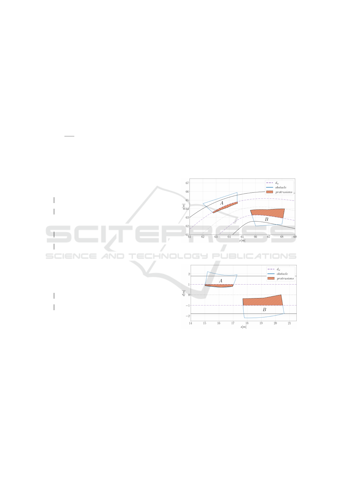
Figure 1: Obstacles A,B (blue) and their protrusions (orange)
in Cartesian coordinates using Algorithm 1.
Figure 2: Obstacles A,B (blue) and their protrusions (orange)
in Frenet frame using Algorithm 1.
Subsequently, we detect the nearest lane boundary
ζ using the minimum d -to-boundary difference in
Frenet frame. ζ and the road’s orientation designate the
clipping direction, with which we carry out a second
iteration of SH at the lane boundary to yield O
sd
, i.e.,
the set of protruded obstacle data points. Note that
O
sd
may contain concave or separate polygons in case
of reverse clipping, and that O
sd
=
/
0 if the obstacle
completely lies outside the lane. We initially handled
the case of non-convex polygons by converting them to
Efficient Real-Time Obstacle Avoidance Using Multi-Objective Nonlinear Model Predictive Control and Semi-Smooth Newton Method
183

convex hulls (again with Graham’s scan), yet this was
abandoned in favor of employing more conservative
safety margins in the envelope functions to achieve
better performance. Overall, Algorithm 1 is quite
efficient, in which determining the protrusions of
the two obstacles A,B illustrated in Figure (1, 2) for
d
w
= 1[m] took only 7.4 × 10
−4
[s] , thus it can handle
a multitude of obstacles in a few milliseconds.
3.2.2 Constructing Envelope Functions
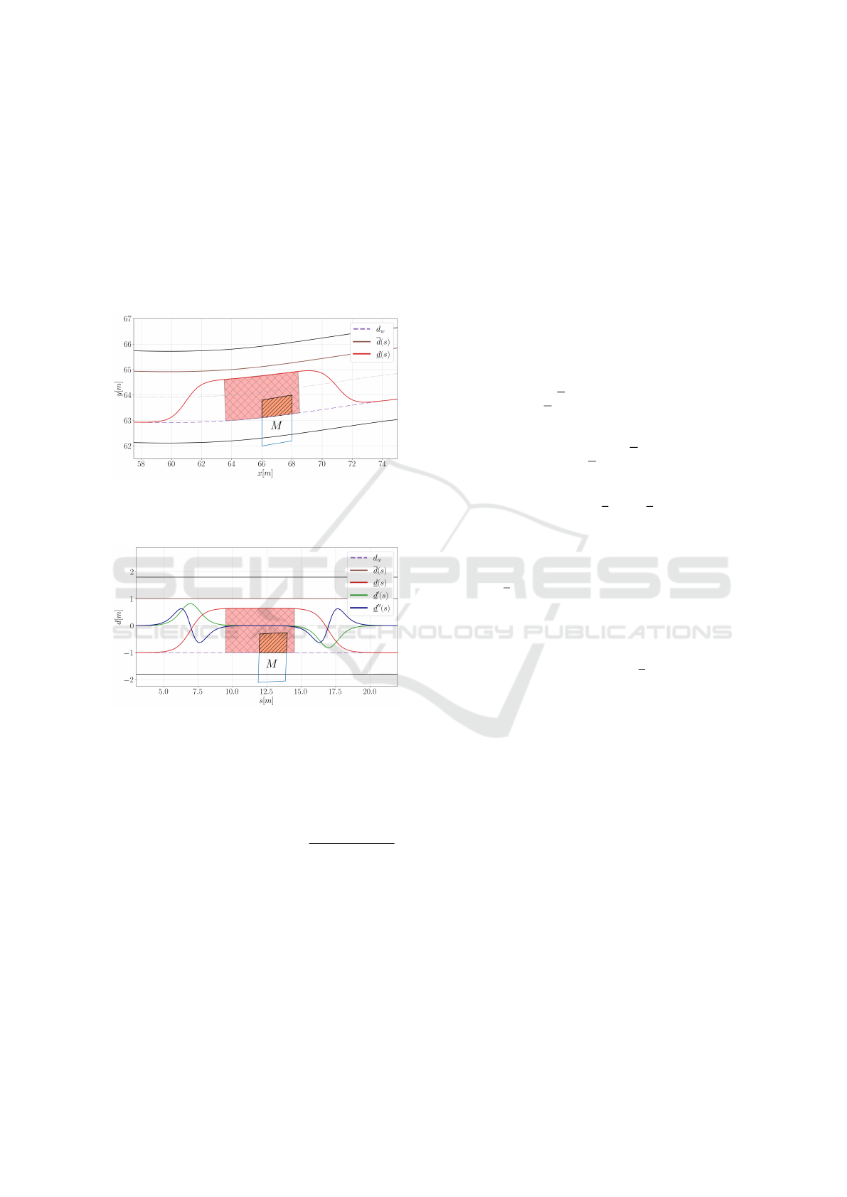
Figure 3: An obstacle with its envelope function in Cartesian
coordinates. The red shaded area is the extended footprint
on account of w, l
b
,l
f
and obstacle-specific safety margins.
Figure 4: An obstacle with its envelope function in Frenet
frame. The function is easily and sufficiently differentiable.
Finally, we compute s
b
,s
f
,d
r
,d
l
from the set of
protrusions O
sd
(similar to Algorithm 1 and derive
a smooth envelope function that entirely captures the
obstacle using logistic functions with:
g(s) := αg
b
(s)g
f
(s), g
b/ f
(s) =
1
1 + exp
−k(s−s
o
)
where k, s
o
are derived from the obstacle’s location
s
b/ f
and the ego-vehicle’s length l
f /b
, and α is derived
from d
r
or d
l
(based on ζ ) and the ego-vehicle’s w .
Depending on the obstacle’s type, parameters α,k,s
o
may also be padded with additional safety margins.
A complete envelope function with its derivatives are
available in Figure (3, 4). Remarkably, the envelope
function g(s) is sufficiently differentiable and has the
nice property that:
g
′
= kg(1 − g), g
′′
= kg
′
(1 − 2g)
i.e., its derivatives can be analytically reached, thus
reducing the computational burden and enabling faster
convergence. Incidentally, a more accurate (yet equally
more demanding) approach to create sufficiently differ-
entiable g(s) would be to apply curve fitting methods
directly to the protrusions O
sd
, e.g., using polynomial
or spline curves (Zhang and Chen, 2022). Unfortu-
nately, this is not only slower, but also mandates having
non-concave protrusions and also -preferably- convex
hulls for obstacles that are too close to each other
so as to avoid overaggressive maneuvering. Imple-
menting and evaluating a curve fitting approach is
hereby deferred for future work.
3.2.3 Handling Obstructed Travel Paths
After computing d,d , we evaluate these functions
across the MPC prediction horizon and inspect if the
travel path is blocked due to one or more obstacles by:
s
h
:= {min(s) ∈ s(t) : d(s) ≥ d(s),t ∈ [0,t
f
]}
where s
h
=
/
0 if no obstacles obstruct the travel path.
Afterwards, we employ a single logistic function to
construct the smooth bound v(s) s.t. v(s
h
) ≈ 0 , which
reduces the maximum allowed velocity to 0 at s
h
. This
can also be utilized to arbitrarily stop the ego-vehicle,
e.g., at traffic lights or at a temporary destination, by
means of a virtual blocking obstacle at a desired ˜s
h
.
Otherwise, v(s) remains constant across the prediction
horizon and is equal to the road speed limit.
To promote passenger comfort and avoid excessive
maneuvering, we utilized different sets of MPC param-
eters ω
∗
for normal driving and stopping. We added
the rigid activation condition max(v(s)) ≤ 2.0[ms
−
1]
and evaluated it at the start of each prediction iteration
to identify the driving mode and accordingly update
ω
∗
for this iteration. This concludes our MPC design
process for path planning and obstacle avoidance.
4 SIMULATION ENVIRONMENT
To properly assess our MPC, it is essential to under-
stand how it fits as a component in a standard archi-
tecture for developing AD systems. Several refer-
ences explain the different hardware and software
elements comprising a functional architecture (Zong
et al., 2018; Parekh et al., 2022; Ziegler et al., 2014),
which we employed as guidelines to identify the key
features required to effectively simulate the developed
controller. These components alongside their commu-
nication channels are summarized in Figure (5) and
will be briefly described in the subsequent sections.
In addition, a prevalent approach in developing AD
features involves preparing the system components as
VEHITS 2024 - 10th International Conference on Vehicle Technology and Intelligent Transport Systems
184

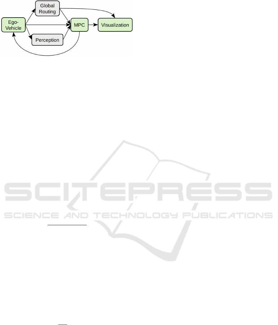
Figure 5: Simplified components of the simulation environ-
ment and their communication channels.
Robot Operating System (ROS) packages. ROS is
an open-source middleware framework for robotics
development and is extensively utilized in diverse
fields, e.g., aviation, automotive, and agriculture
(Quigley et al., 2009). Accordingly, we developed
the simulation environment components as separate
software packages in order to facilitate their migration
to ROS in the future.
4.1 Ego-Vehicle
The first component is the motion model that suitably
simulates the dynamical behavior of the ego-vehicle
based on the received control action from the MPC.
Herein, we offer two models defined in different
coordinate systems to ensure the flexibility of our
approach: first, a nonlinear version of the point-mass
vehicle model in Frenet frame relative to a reference
path (Emam and Gerdts, 2022):
s
′
(t) =
v(t) cos χ(t)
1 − d(t)κ
r
(s(t))
d
′
(t) = v(t)sinχ(t)
χ
′
(t) = v(t)κ(t) − s
′
(t)κ
r
(s(t))
κ
′
(t) = u
1
(t)
v
′
(t) = u
2
(t)
(17)
with the same state and input vectors as (15). Second, a
simplified single-track (kinematic) model in Cartesian
coordinates (Burger and Gerdts, 2019):
x
′
(t) = v(t)cosϕ(t)
y
′
(t) = v(t)sinϕ(t)
ϕ
′
(t) =
v(t)
l
f
tanδ(t)
δ
′
(t) = l
f
u
1
(t)cos
2
δ(t)
v
′
(t) = u
2
(t)
(18)
with the states: (x,y) the position of the ego-vehicle,
ϕ its yaw angle, δ its steering angle, and v its velocity.
The model has the inputs: steering rate w
δ
and
acceleration, in which w
δ
is determined from the MPC
input κ
′
= u
1
with the mapping w
δ
(t) = ℓu(t)cos
2
δ(t)
(Britzelmeier and Gerdts, 2020).
After each MPC solution iteration, we use the
computed controls and employ a Runge-Kutta (RK4)
method on the selected system model to accurately
calculate the updated vehicle position, heading, and
velocity at any desired time. The nonlinearities in both
models ensure that the vehicle states are different from
the MPC predictions each iteration, which mimics the
process of deploying the controller on real hardware.
This component will be substituted with the actual
vehicle equipped with sensors and actuator modules
that can apply the MPC controls and update the vehicle
states accordingly.
4.2 Global Routing
This package is responsible for traversing the road
network to identify a feasible travel path γ
re f
between
the current ego-vehicle position and the desired desti-
nation as selected by the passenger. This can be
achieved by means of, for example, a combination
of A* or Dijkstra algorithms (Qin et al., 2023) and
OpenStreetMap (OSM) data (OpenStreetMap contrib-
utors, 2017). This is a high-level task that a navigation
system traditionally performs, and is stubbed in our
simulation environment with a pre-defined reference
path data, which is transmitted to the controller at the
beginning of the simulation.
4.3 Perception
Perception is an umbrella term for environment anal-
ysis objectives, like: traffic signs recognition, object
detection and tracking, sensor data processing and
fusion, and many more (Parekh et al., 2022). Generally,
it comprises several modules, which are responsible
for building task-oriented world models to cater to the
different system DDTs (Zhang et al., 2023). Due to
its complexity, we implement a mock version, which
simply transmits pre-defined positions and orientations
of static obstacles located across the travel path to
emulate an obstacle avoidance scenario.
4.4 MPC
We prepared the developed controller as a software
package that receives the global path data, positions
and orientations of obstacles, and relevant ego-vehicle
states (e.g., position and velocity). Subsequently, the
MPC solves the DOCP and determines the optimal
control action, which is then transferred back to
the ego-vehicle component to initiate its movement.
Furthermore, the control action and other important
Efficient Real-Time Obstacle Avoidance Using Multi-Objective Nonlinear Model Predictive Control and Semi-Smooth Newton Method
185

data, such as the local planned travel path and the
DOCP solution time, are transmitted to the visualiza-
tion component for data collection and monitoring.
4.5 Visualization
Lastly, this helper package was implemented to facil-
itate gathering and displaying all relevant problem
information. This includes the global reference path,
the vehicle states, the iterative DOCP travel path and
solution time, and so on. The package is used in the
numerical simulation and in performance assessment
of the developed controller.
5 NUMERICAL TESTING AND
RESULTS
After laying out the components of the OCP solver
and simulation environment, we implemented them
entirely in C++ and recorded the simulation results
on a Linux system with the processor i5-5200U of
2.20GHz and 8GB of RAM. For problem discretiza-
tion, we utilized the trapezoidal rule, and for the
MPC parameters, we selected a prediction horizon
of ∆T = 4.5[s] with N = 30 control points and a time
step of T
s
= 0.15[s] . The objective function weights
were initially selected based on the scaled contribution
of system states and controls, then slightly modified
using trial and error.
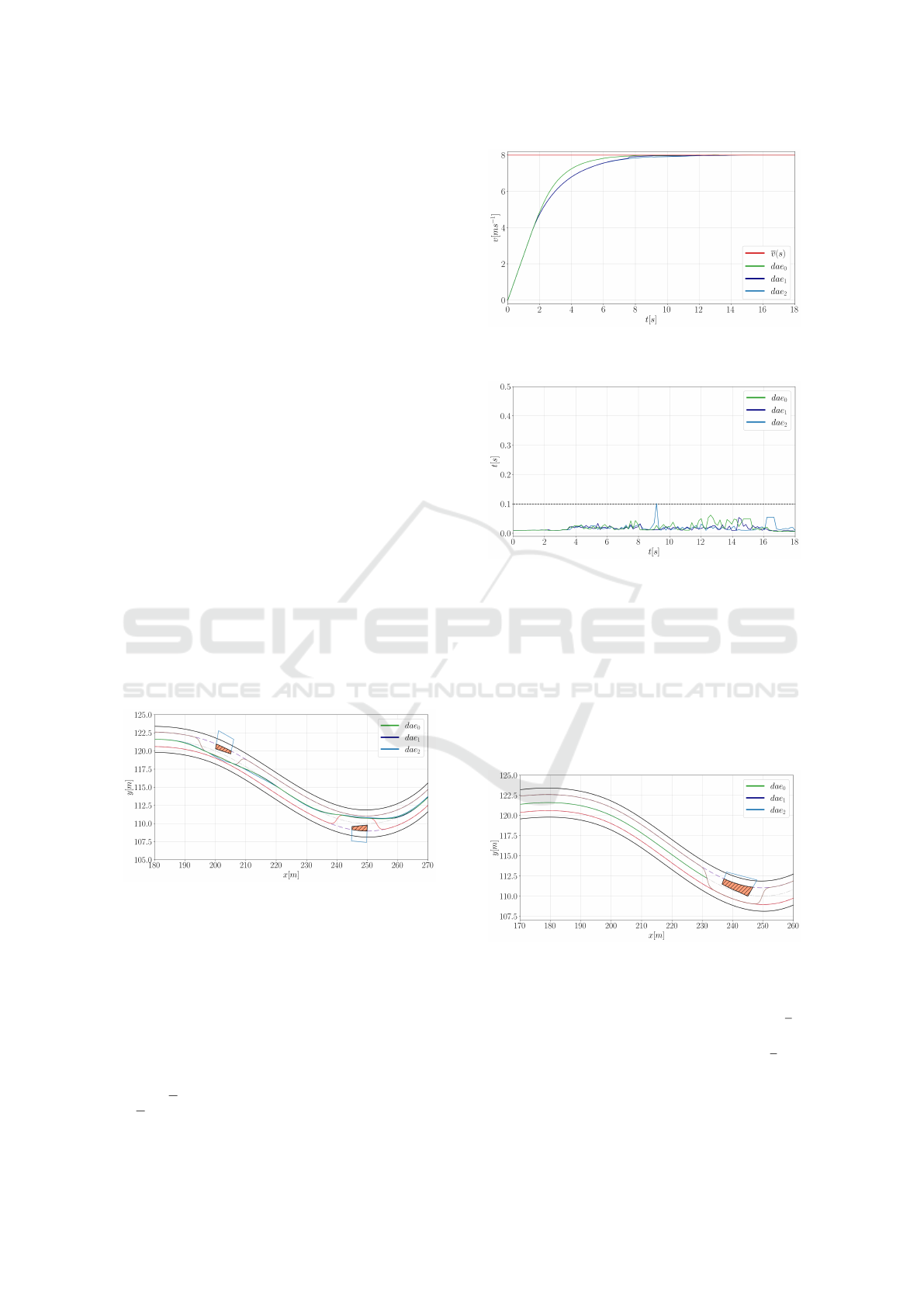
Figure 6: Path following with obstacle avoidance is success-
fully completed on a highly dynamic road.
We developed and executed two scenarios to
highlight our DDTs, i.e., path tracking with obstacle
avoidance and a braking maneuver in case of full road
obstruction. Each scenario was simulated three times
with the linear (15) and nonlinear (17), (18) motion
models, which are denoted in the upcoming figures as
dae
0
,dae
1
,dae
2
respectively. Also, we proceed with
the same color palette for marking the reference path,
driving lane, and admissible driving area on account
of (d(s),d(s)).
Figure 7: Velocity trajectories of the motion models in the
first test scenario.
Figure 8: Solution time of the DOCPs in the first scenario.
In the first test scenario, the ego-vehicle starts
moving from standstill and is able to successfully
maneuver between two stationary obstacles on either
side of its travel path as demonstrated in Figure
(6). Slight variations between the motion models are
noticeable, which is expected due to their different
dynamical behaviors. The vehicle controls are properly
mapped and minimal execution time is required to
reach on optimal solution, cf. Figure (8).
Figure 9: The ego-vehicle brakes properly in case of a fully
obstructed path.
In the second scenario, the ego-vehicle starts with
v = 6[ms
−1
] and accelerates at first to reach v =
8[ms
−1
] before it recognizes that its travel path is
obstructed. Accordingly, the smooth function v(s) is
constructed and the vehicle decelerates and adequately
stops behind the blocking obstacle as illustrated in
Figure (9). Notice that the execution time marginally
VEHITS 2024 - 10th International Conference on Vehicle Technology and Intelligent Transport Systems
186

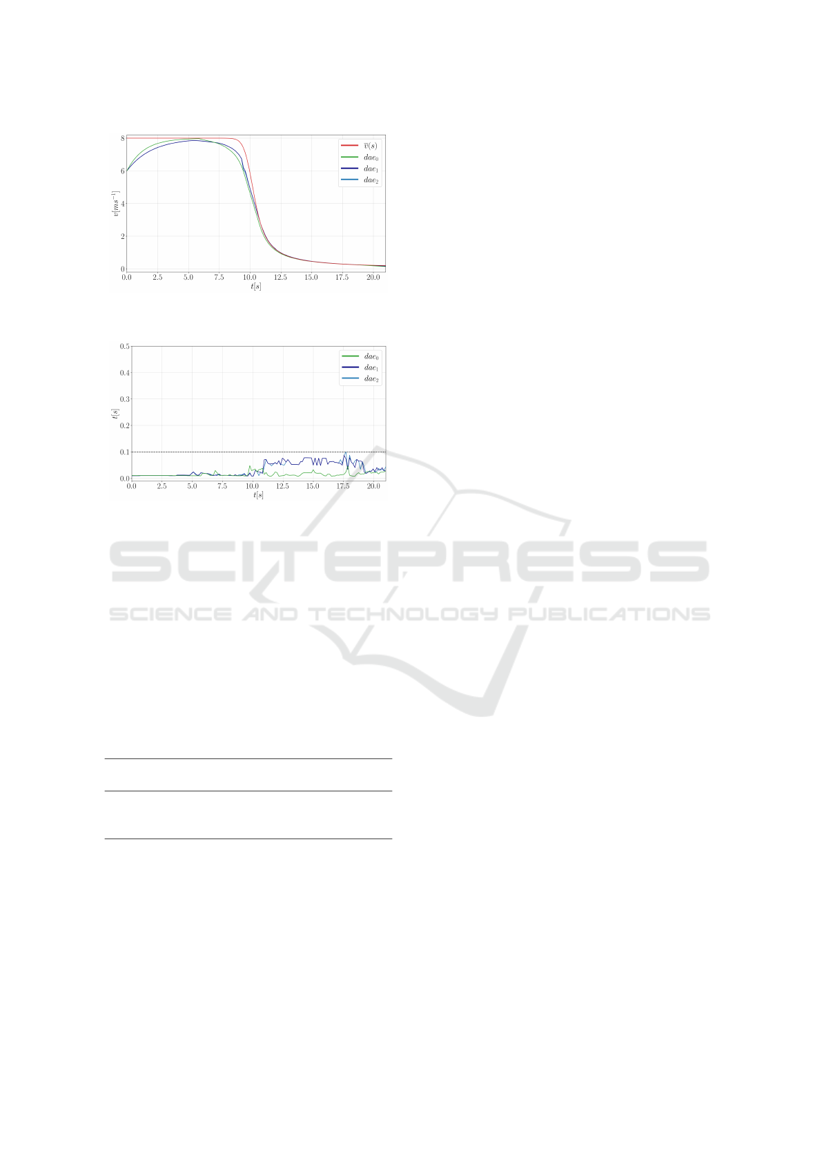
Figure 10: Velocity trajectories of the motion models in the
second test scenario.
Figure 11: Solution time of the DOCPs in the second
scenario.
increases in the second segment of the test scenario,
i.e., after t = 11.0[s] , which is due to attempting to
travel at a considerably low speed. This leads to
ill-conditioning of the DOCP, which unnecessarily
increases the computational time and can be remedied
by refining the braking/stopping MPC parameters ω
∗
.
Alternatively, a simpler controller (e.g., PID) can be
developed and configured to halt the ego-vehicle, and
a hybrid strategy can be introduced to switch between
both controllers based on the driving situation.
Table 1: Average and maximum solution times (in seconds)
for both test scenarios.
Scenario 1 Scenario 2
mean max mean max
dae
0
0.01982 0.06214 0.01582 0.04817
dae
1
0.01577 0.05378 0.03425 0.08739
dae
2
0.01796 0.10132 0.03424 0.09987
We highlight that in both test scenarios the MPC
controller is almost always able to compute a feasible
solution under 100[ms] , cf. Table (1). This, coupled
with its high update rate and appropriate prediction
horizon, is sufficient to satisfy the real-time require-
ment for a typical autonomous driving application.
Lastly, an important point to discuss is that MPC
controllers are problem-specific, so it is quite chal-
lenging to compare them to each other, even for
the same DDT. For example, (Gutjahr et al., 2017;
Britzelmeier and Gerdts, 2020) use MPC for obstacle
avoidance, where they utilize a linear MPC for lateral
vehicle control with independent longitudinal control.
We, however, tackle a DOCP with coupled lateral and
longitudinal controls. Moreover, (Zhang and Chen,
2022; Wang and Liu, 2022) generate collision-free
travel paths using RRT* and A* algorithms, then
employ MPC controllers for path following. Yet,
our approach embeds the path generation aspect in
the controller itself, in addition to handling fully
obstructed travel paths. For more examples on MPC
in AD applications, we refer the reader to (Musa et al.,
2021).
6 CONCLUSION AND FUTURE
WORK
In this work, we discussed the development process
and successful deployment of an efficient NMPC
controller to achieve real-time path planning and
obstacle avoidance for autonomous vehicles. First, we
extended a previously proposed semi-smooth Newton
method to accommodate nonlinear DOCPs. Second,
we elaborated on MPC development for path plan-
ning, while introducing a numerically efficient object
projection algorithm that allows for obstacle incorpo-
ration and simplifies the problem constraints to guar-
antee faster solution convergence. Finally, we imple-
mented a simulation environment and assessed the
performance of the developed controller for different
motion models, and in driving situations that mimic
reality.
Ideas for future work include developing a high-
fidelity vehicle model to more accurately simulate the
vehicle dynamics and further expedite the controller
development and tuning by minimizing the reliance
on actual test vehicles. As for obstacle avoidance,
adapting our proposed algorithm to handle dynamic
objects and/or multiple driving lanes, as well as
investigating a curve-fitting approach for more realistic
safety margins, are intriguing prospects. Finally, we
conclude our suggestions with a full migration of the
controller to ROS and its integration and deployment
on actual hardware. Nonetheless, this will require
thorough testing and optimization to ensure that the
real-time requirement still upholds.
Efficient Real-Time Obstacle Avoidance Using Multi-Objective Nonlinear Model Predictive Control and Semi-Smooth Newton Method
187

ACKNOWLEDGEMENTS
This research paper is part of [project MORE – Munich
Mobility Research Campus] and funded by dtec.bw
– Digitalization and Technology Research Center of
the Bundeswehr. dtec.bw is funded by the European
Union – NextGenerationEU.
REFERENCES
Britzelmeier, A. and Gerdts, M. (2020). A nonsmooth
newton method for linear model-predictive control
in tracking tasks for a mobile robot with obstacle
avoidance. IEEE Control Systems Letters, PP:1–1.
Burger, M. and Gerdts, M. (2019). DAE Aspects in Vehicle
Dynamics and Mobile Robotics, pages 37–80. Springer
International Publishing, Cham.
Chachuat, B. (2007). Nonlinear and dynamic optimization:
From theory to practice.
Chen, X., Nashed, Z., and Qi, L. (2000). Smoothing methods
and semismooth methods for nondifferentiable oper-
ator equations. SIAM Journal on Numerical Analysis,
38(4):1200–1216.
Clarke, F. H. (1990). Optimization and Nonsmooth Anal-
ysis. Society for Industrial and Applied Mathematics
(SIAM), Philadelphia, USA.
Diehl, M., Bock, H. G., and Schl
¨
oder, J. P. (2005). A real-
time iteration scheme for nonlinear optimization in
optimal feedback control. SIAM Journal on Control
and Optimization, 43(5):1714–1736.
Emam, M. and Gerdts, M. (2022). Deterministic operating
strategy for multi-objective nmpc for safe autonomous
driving in urban traffic. In Proceedings of the 8th
International Conference on Vehicle Technology and
Intelligent Transport Systems - VEHITS, pages 152–
161.
Emam, M. and Gerdts, M. (2023). Sensitivity updates
for linear-quadratic optimization problems in multi-
step model predictive control. Journal of Physics:
Conference Series, 2514(1):012008.
Fischer, A. (1992). A special newton-type optimization
method. Optimization, 24(3-4):269–284.
Gerdts, M. (2023). Optimal control of ODEs and DAEs. De
Gruyter Oldenbourg, Munich, Germany, 2 edition.
Gerdts, M. and Kunkel, M. (2008). A nonsmooth newton’s
method for discretized optimal control problems with
state and control constraints. Journal of Industrial &
Management Optimization, 4(2):247–270.
Gerdts, M. and Kunkel, M. (2009). A globally conver-
gent semi-smooth newton method for control-state
constrained dae optimal control problems. Computa-
tional Optimization and Applications, 48(3):601–633.
Graham, R. (1972). An efficient algorith for determining
the convex hull of a finite planar set. Information
Processing Letters, 1(4):132–133.
Gr
¨
une, L. and Pannek, J. (2011). Nonlinear Model Predictive
Control: Theory and Algorithms. Communications and
Control Engineering. Springer, London, England.
Gutjahr, B., Gr
¨
oll, L., and Werling, M. (2017). Lateral
vehicle trajectory optimization using constrained linear
time-varying mpc. IEEE Transactions on Intelligent
Transportation Systems, 18(6):1586–1595.
Harwood, D. W. and Mason, J. M. (1994). Horizontal curve
design for passenger cars and trucks. Transportation
Research Record.
Hoss, M., Scholtes, M., and Eckstein, L. (2022). A review of
testing object-based environment perception for safe
automated driving. Automotive Innovation, 5(3):223–
250.
Hughes, J. F., McGuire, M. S., Foley, J., Sklar, D. F., Feiner,
S. K., Akeley, K., Van Dam, A., and Foley, J. D. (2009).
Computer Graphics: Principles and Practice. Addison-
Wesley Educational, Boston, MA, 3 edition.
Jiang, H. (1999). Global convergence analysis of the general-
ized newton and gauss-newton methods of the fischer-
burmeister equation for the complementarity problem.
Mathematics of Operations Research, 24(3):529–543.
Jiang, H. and Qi, L. (1997). A new nonsmooth equa-
tions approach to nonlinear complementarity problems.
SIAM Journal on Control and Optimization, 35(1):178–
193.
Jiang, H. and Ralph, D. (1998). Global and Local
Superlinear Convergence Analysis of Newton-Type
Methods for Semismooth Equations with Smooth Least
Squares, pages 181–209. Springer US.
Morari, M. and H. Lee, J. (1999). Model predictive control:
past, present and future. Computers & Chemical
Engineering, 23(4–5):667–682.
Musa, A., Pipicelli, M., Spano, M., Tufano, F., De Nola,
F., Di Blasio, G., Gimelli, A., Misul, D. A., and
Toscano, G. (2021). A review of model predictive
controls applied to advanced driver-assistance systems.
Energies, 14(23).
OpenStreetMap contributors (2017). Planet dump retrieved
from https://planet.osm.org . https://www.openstreet
map.org.
Palma, V. G. (2015). Robust Updated MPC Schemes. PhD
thesis, Universit
¨
at Bayreuth, Bayreuth.
Parekh, D., Poddar, N., Rajpurkar, A., Chahal, M., Kumar,
N., Joshi, G. P., and Cho, W. (2022). A review
on autonomous vehicles: Progress, methods and
challenges. Electronics, 11(14):2162.
Qin, H., Shao, S., Wang, T., Yu, X., Jiang, Y., and Cao,
Z. (2023). Review of autonomous path planning
algorithms for mobile robots. Drones, 7(3):211.
Quigley, M., Conley, K., Gerkey, B. P., Faust, J., Foote, T.,
Leibs, J., Wheeler, R., and Ng, A. Y. (2009). Ros:
an open-source robot operating system. In ICRA
Workshop on Open Source Software.
Rawlings, J. B. and Mayne, D. Q. (2009). Model Predictive
Control: Theory and Design. Nob Hill Pub, LLC,
California, USA.
Sussmann, H. and Willems, J. (1997). 300 years of optimal
control: From the brachystochrone to the maximum
principle. IEEE Control Systems, 17(3):32–44.
Sutherland, I. E. and Hodgman, G. W. (1974). Reentrant
polygon clipping. Communications of the ACM,
17(1):32–42.
VEHITS 2024 - 10th International Conference on Vehicle Technology and Intelligent Transport Systems
188

Ulbrich, M. (2002). Semismooth newton methods for
operator equations in function spaces. SIAM Journal
on Optimization, 13(3):805–841.
Vu, T. M., Moezzi, R., Cyrus, J., and Hlava, J. (2021). Model
predictive control for autonomous driving vehicles.
Electronics, 10(21):2593.
Wang, H. and Liu, B. (2022). Path planning and path tracking
for collision avoidance of autonomous ground vehicles.
IEEE Systems Journal, 16(3):3658–3667.
Zhang, D. and Chen, B. (2022). Path planning and predictive
control of autonomous vehicles for obstacle avoidance.
In 2022 18th IEEE/ASME International Conference on
Mechatronic and Embedded Systems and Applications
(MESA). IEEE.
Zhang, Y., Carballo, A., Yang, H., and Takeda, K. (2023).
Perception and sensing for autonomous vehicles under
adverse weather conditions: A survey. ISPRS Journal
of Photogrammetry and Remote Sensing, 196:146–177.
Ziegler, J., Bender, P., Dang, T., and Stiller, C. (2014).
Trajectory planning for bertha - a local, continuous
method. In 2014 IEEE Intelligent Vehicles Symposium
Proceedings. IEEE.
Zong, W., Zhang, C., Wang, Z., Zhu, J., and Chen, Q.
(2018). Architecture design and implementation of
an autonomous vehicle. IEEE Access, 6:21956–21970.
Efficient Real-Time Obstacle Avoidance Using Multi-Objective Nonlinear Model Predictive Control and Semi-Smooth Newton Method
189