Parameter Adjustments in POMDP-Based Trajectory Planning for

Unsignalized Intersections

Adam Kollar

ık

1,2 a

and Zden

ek Hanz

alek

2 b

Dept. of Control Engineering, Faculty of Electrical Engineering, Czech Technical University in Prague, Czech Republic

Czech Institute of Informatics, Robotics and Cybernetics, Czech Technical University in Prague, Czech Republic

Keywords:

Automated Intersection Crossing, Trajectory Planning, POMDP.

Abstract:

This paper investigates the problem of trajectory planning for autonomous vehicles at unsignalized intersec-

tions, speciﬁcally focusing on scenarios where the vehicle lacks the right of way and yet must cross safely. To

address this issue, we have employed a method based on the Partially Observable Markov Decision Processes

(POMDPs) framework designed for planning under uncertainty. The method utilizes the Adaptive Belief Tree

(ABT) algorithm as an approximate solver for the POMDPs. We outline the POMDP formulation, beginning

with discretizing the intersection’s topology. Additionally, we present a dynamics model for the prediction of

the evolving states of vehicles, such as their position and velocity. Using an observation model, we also de-

scribe the connection of those states with the imperfect (noisy) available measurements. Our results conﬁrmed

that the method is able to plan collision-free trajectories in a series of simulations utilizing real-world trafﬁc

data from aerial footage of two distinct intersections. Furthermore, we studied the impact of parameter adjust-

ments of the ABT algorithm on the method’s performance. This provides guidance in determining reasonable

parameter settings, which is valuable for future method applications.

1 INTRODUCTION

The advent of autonomous vehicles signals a change

in urban mobility, promising to enhance efﬁciency,

safety, and the overall driving experience. One of the

challenges these vehicles face is crossing an unsignal-

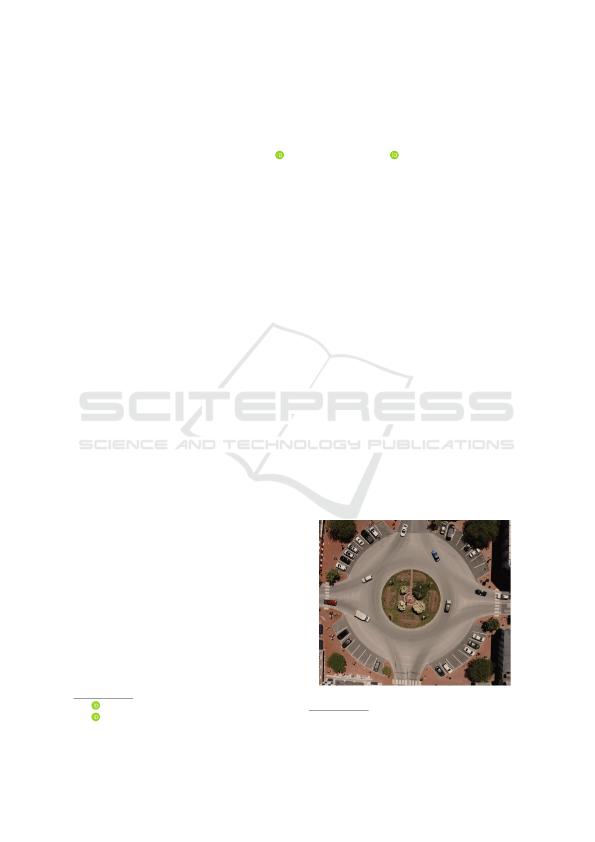
ized intersection, e.g., a roundabout shown in Fig-

ure 1. With the absence of trafﬁc signals and espe-

cially without the right of way, the autonomous ve-

hicle must independently determine whether and how

to proceed, guided only by trafﬁc regulations and the

inherently uncertain behavior of other vehicles, per-

ceived by measurements affected by noise. This is

the description of the trajectory planning problem for

unsignalized intersections we explore in this paper.

In particular, we investigate a method based

on Partially Observable Markov Decision Processes

(POMDPs), a framework for planning under uncer-

tainty with incomplete information. For a given inter-

section and 2D measurements of other vehicles, the

method outputs the trajectory as a sequence of accel-

erations along the desired path.

https://orcid.org/0000-0002-9150-839X

https://orcid.org/0000-0002-8135-1296

Our contributions are twofold. At ﬁrst, we verify

the capability of the POMDP-based method to plan

collision-free trajectories in simulations using real-

life trafﬁc data from aerial footage of two intersec-

tions with different topologies

. In addition, based on

those simulations, we analyze the inﬂuence of the pa-

rameter values on the method’s performance.

Figure 1: Unsignalized intersection (roundabout).

See our supplementary YouTube video.

522

Kollar

cík, A. and Hanzálek, Z.

Parameter Adjustments in POMDP-Based Trajectory Planning for Unsignalized Intersections.

DOI: 10.5220/0012742400003702

Paper published under CC license (CC BY-NC-ND 4.0)

In Proceedings of the 10th International Conference on Vehicle Technology and Intelligent Transport Systems (VEHITS 2024), pages 522-529

ISBN: 978-989-758-703-0; ISSN: 2184-495X

2 RELATED WORK

The literature (Eskandarian et al., 2021; Hubmann

et al., 2018) broadly divides the planning strategies

for automated vehicles into rule-based, reactive, and

interactive methods, each with distinct approaches to

predicting future events.

The rule-based methods have a predeﬁned set

of rules and actions established (Schwarting et al.,

2018), e.g., in the form of a ﬁnite state machine. Thus

their decisions rely only on the current state. The re-

active methods treat the motion of vehicles as inde-

pendent entities. They may introduce simplifying as-

sumptions such as the constant velocity of other ve-

hicles or their set future behavior (Hubmann et al.,

2018). Together with the rule-based methods, they

lack the ability to consider the interconnected behav-

ior of all vehicles, which is essential for safe interac-

tions in automated driving (Schwarting et al., 2018).

Interactive methods can be either centralized or

decentralized (Eskandarian et al., 2021). The cen-

tralized methods are usually based on the Vehicle-to-

Everything (V2X) paradigm (Tong et al., 2019) and

assume communication among vehicles to generate

a single global strategy. Nevertheless, given predic-

tions that only half of the vehicles will be autonomous

by 2060 (Litman, 2023), decentralized approaches

are vital for the foreseeable future. Decentralized

methods might be further categorized into three main

groups according to their way of tackling interactiv-

ity. Those are game theory-based, probabilistic, and

data-driven approaches (Schwarting et al., 2018).

This paper investigates a probabilistic planning

method developed for unsignalized intersection cross-

ing introduced in (Hubmann et al., 2018) based on

POMDPs. The method relies on the Adaptive Belief

Tree algorithm (Kurniawati and Yadav, 2016), using

a particle ﬁlter to estimate the probability distribu-

tion of non-observable variables, such as the inten-

tions of other vehicles. In (Bey et al., 2021), the

authors employed the method for driving at round-

abouts. In (Hubmann et al., 2019), occlusion caused

both by the environment and by other dynamic ob-

jects was included, and in (Schulz et al., 2019), an

improved behavior prediction with dynamic Bayesian

network was introduced.

3 APPROACH

This section outlines the components of our approach

to addressing the unsignalized intersection crossing

problem. We begin by providing a formal problem

deﬁnition in Section 3.1. Key to our strategy is for-

mulating this problem as a POMDP, which we dis-

cuss in Section 3.2. To solve the POMDP, we ap-

ply an approximate solver called the Adaptive Belief

Tree (ABT) algorithm, detailed in Section 3.3. Our

method involves discretizing the intersection topol-

ogy, a process explained in Section 3.4, where we

identify all feasible 2D paths without lane changes

based on combinations of intersection entrances and

exits. Subsequently, we introduce dynamical and ob-

servation models in Sections 3.5, and 3.6, respec-

tively, that capture the complexities of the real world

in a simpliﬁed yet sufﬁciently accurate manner for tra-

jectory planning. Entities such as state and observa-

tion are deﬁned, and we construct a reward function

in Section 3.7. This function is designed to be max-

imized within the POMDP, ensuring that the result-

ing trajectory aligns with our expectations, e.g., en-

compasses crucial factors such as collision avoidance

and adherence to velocity limits. To complete the pro-

cess, we leverage the mentioned ABT solver for our

POMDP formulation to derive the desired trajectory

as a sequence of longitudinal accelerations along the

desired path toward the goal exit of the intersection.

3.1 Formal Problem Deﬁnition

To formally deﬁne the problem, we seek a collision-

free trajectory through a known intersection topology

along a predeﬁned path φ

φ(t) : t → R

, t ∈ [0, d] where

d is the total length of the path. We assume that

the position p

= [x

, y

]

⊤

, velocity v

= [v

x,i

, v

y,i

]

⊤

unit heading vector θ

, width w

, and length l

mea-

surements of all n relevant other (non-ego) vehicles

i ∈ {1, ...,n} are available every sample time k. Thus,

we are looking for a sequence of longitudinal accel-

erations a

of the ego vehicle (denoted with the zero

subscript), such that there is no overlap between the

bounding rectangles given by p

, θ

, w

, l

and p

, w

, l

for each i. Lateral accelerations of all ve-

hicles need not to be directly determined, as the cur-

vature of the followed path implicitly controls it, pro-

vided that drifting is avoided.

3.2 POMDPs

POMDPs generalize the Markov Decision Process

(MDP) framework for decision-making and planning

under uncertainty (Kurniawati, 2022). They are de-

ﬁned by a tuple

⟨

S,A,O,T,Z,R,γ

⟩

, where S is the set

of states, A is a set of actions, O is the set of obser-

vations, T is a set of conditional transition probabili-

ties between states, Z is a set of conditional observa-

tion probabilities, R : S ×A is the reward function, and

γ ∈ (0, 1] is the discount factor.

Parameter Adjustments in POMDP-Based Trajectory Planning for Unsignalized Intersections

523

Fundamentally, T represents the stochastic dy-

namics model of the system, and Z represents the

stochastic observation (measurement) model with the

probabilities T (s

′

|a,s) of transition from state s ∈ S to

state s

′

∈ S with action a ∈ A, and Z(o|a,s

′

) of obser-

vation o ∈ O in s

′

. The particular way of modeling the

dynamical and measurement properties for our pur-

poses is described Sections 3.5 and 3.6.

Since the current state is unknown, the belief

b ∈ B is introduced, representing a distribution over

all states from the set B known as the belief space:

b(s

′

) ∝ Z(o | a,s

′

)

∑

s∈S

T (s

′

| a, s)b(s), (1)

where ∝ denotes that the right-hand side probabil-

ities are not normalized. This converts the origi-

nal POMDP problem into an MDP where beliefs are

states, with continuous and observable state space B.

The goal of the POMDP planner is to determine a

policy π : B → A, that maximize the expected sum of

discounted rewards called the value function V :

V = E

∞

∑

k=0

R(s

)



b,π

. (2)

Even though the belief space is continuous, exact

POMDP solvers exist. They are based on the fact

that any optimal value function is piecewise linear and

convex and thus can be described as an upper enve-

lope of a ﬁnite set of linear functions called the α-

vectors (Braziunas, 2003). Nevertheless, exact meth-

ods are highly intractable and not suitable for on-

line applications (Kurniawati, 2022). Approximate

online methods mostly perform a belief tree search

combining heuristics, branch and bound pruning, and

Monte Carlo sampling (Ye et al., 2017). An example

of these approximate methods is the Adaptive Belief

Tree algorithm (ABT) implemented with its variants

in a publicly available solver called TAPIR (Klimenko

et al., 2014), which we use in our work.

3.3 Adaptive Belief Tree Algorithm

The ABT algorithm (Kurniawati and Yadav, 2016) is

an online and anytime POMDP solver that uses the

Augmented Belief Tree for ﬁnding well-performing

policies. The tree T is constructed by sampling ini-

tial belief b

with n

par

particles and propagating them

with actions according to the observation and dynam-

ics models T and Z until the set depth of the optimiza-

tion horizon N or a terminal state is reached. At each

step, the particles are assigned a reward r = R(s, a).

Sequences of quadruples (s

) representing

a path in the tree where i is the depth of each contained

Figure 2: Illustrative example of an augmented belief tree.

node are sampled state trajectories also referred to as

episodes. At last, each episode is assigned a quadru-

ple (s

,−,−, r

) where s

is a sampled next state

and r

is the expected future reward for the follow-

ing states. This is computed directly for the terminal

states; non-terminal states are heuristically estimated,

in our case, with a 3-step lookahead. An example of

an Augmented Belief Tree is illustrated in Figure 2.

With the tree containing n

episodes, the policy

based on a Q(b,a) (Q-value) estimate

Q(b,a) for each

belief-action pair is obtained:

V (b,π) = max

a∈T (b)

Q(b,a), (3)

π(b) = argmax

a∈T (b)

Q(b,a), (4)

where Q(b,a) is the reward for performing an action a

in the ﬁrst step and then behaving optimally. The esti-

mate is computed as an average reward of all episodes

h ∈ H(b,a) containing the pair (b,a) in depth l:

Q(b,a) =

|H(b,a)|

∑

h∈H(b,a)

∑

i=l

i−l

. (5)

After the action from π(b) is applied and new obser-

vation observed, a particle ﬁlter update according to

(1) is performed, and relevant parts of the tree T are

reused in the next step.

The estimation

Q(b,a) is used not only for deter-

mining the policy π(b) but also during the construc-

tion of the tree T to select the actions for propagat-

ing particles. First, actions that have not been picked

already for the belief are chosen randomly with uni-

form distribution. When there are no unused actions

left, the upper conﬁdence bound (UCB) is employed

to address the exploration-exploitation trade-off:

sel

= argmax

a∈A

Q(b,a) + c

log

∑

|H(b,a)|

, (6)

where c is the tunning UCB parameter.

VEHITS 2024 - 10th International Conference on Vehicle Technology and Intelligent Transport Systems

524

The current belief is updated after the action π(b

)

is applied, and new measurements are obtained. The

corresponding branches of the belief tree are reused,

with the current belief being the new root of the tree.

This process is repeated until the goal is reached. If

needed, new particles are generated to maintain the

par

number of particles to avoid particle depletion.

3.4 Topology Discretization

To simplify the representation of the intersection

within the POMDP and to reduce computational de-

mands, we adopt an approach from (Hubmann et al.,

2018). The intersection is condensed into a set of all

possible paths, as illustrated in Figure 3. Particularly

effective for unsignalized intersections, where only a

few paths are reasonable to assume, this approach re-

duces the description of any vehicle to a triplet of val-

ues s

= [p

, v

, µ

]

⊤

, where µ ∈ {1, ..., m} is the in-

tended path out of the m possible paths, p is the posi-

tion along the path p, and v is the longitudinal veloc-

ity. The state of our POMDP is then represented by a

vector s

s containing these values for all n + 1 vehicles,

including the ego vehicle.

To identify possible paths, we utilize the lanelet2

(Poggenhans et al., 2018) map in the OSM XML for-

mat as a source for the full intersection topology. Us-

ing the lanelet2 library, we generate a route graph,

searching for all possible paths as a sequence of R

points. Subsequently, each path is stored as two sep-

arate cubic splines for the x and y coordinates. This

provides an efﬁcient mapping from the path position

to the global coordinates, denoted as φ

φ(p) : p → R

and mapping to the unit heading ψ

ψ(p) : p → y

y ∈ R

∥y

y∥ = 1. For the inverse mapping converting global

coordinates back to the position on a path, denoted as

ε(p

p) : p

p → R, we employ a search algorithm to deter-

mine the nearest point on the selected path.

3.5 Dynamics Model

As we proceed with the formulation of our POMDP, it

is crucial to introduce a dynamical model describing

how the state, deﬁned in the previous section, evolves

over time. While various mathematical models of dif-

ferent complexities exist for vehicles, we aim for sim-

plicity and reduced computational demand. Thus, we

follow the approach from (Hubmann et al., 2018) and

adopt a discrete linear point mass model for each ve-

hicle i ∈ {0, ..., n}:

k+1

= A

+ B

s) + η

η, η

η ∼ N (0

0,Q

Q), (7)

A =





1 ∆t 0

0 1 0

0 0 1





, B

B =





∆t





. (8)

Here, ∆t represents the time between subsequent sam-

ples k and k + 1, and u(s

s) denotes the acceleration of

the vehicle. The Gaussian noise η

η with zero mean and

covariance matrix Q

Q accounts for model inaccuracies.

The ﬁrst two rows of the model matrices A

A, B

B rep-

resent the change of position p

and velocity v

time. Upon further inspection, it is also noticeable

from their last row that the intention µ

remains con-

stant. Yet, it is unknown for all vehicles except for the

ego. The same applies to acceleration values, which

need to be predicted to estimate the future movement

of the other vehicles.

In (Hubmann et al., 2018), the authors used a

heuristically chosen deceleration when a crash is

anticipated for other vehicles, otherwise, the ref-

erence velocity is followed. Alternatively, a dy-

namic Bayesian network prediction is presented in the

follow-up paper (Schulz et al., 2019). Another ap-

proach (Bey et al., 2021) introduces a version of the

intelligent driver model (IDM) (Treiber et al., 2000).

We implemented the IDM model for its simplicity:

= a

max

IDM

+ ω

, ω

∼ N (0,σ

), (9)

where a

max

is the maximal acceleration, and ω

intro-

duces randomness into the model with variance σ

The factor ρ

IDM

is given by the IDM:

IDM

= 1 −



des



−



∗

lead

)

lead



, (10)

∗

lead

) = d

min

+ v

τ +

− v

lead

)

max

min

, (11)

where v

des

is the desired velocity, τ is the time head-

way, δ is the acceleration exponent, v

lead

is the veloc-

ity of the leading (approached) vehicle, and a

min

is the

minimal acceleration (maximal deceleration).

The acceleration of the ego vehicle is obtained

from the resulting POMDP policy according to (4).

The model (7), and (8) together with other vehicles

acceleration predictions (9) represent the dynamics

model referred to as T in Section 3.2.

3.6 Observation Model

Having established the dynamics model, our focus

shifts to the observation model, describing how the

observations are obtained from the state of the sys-

tem. In this context, observations should align with

measurements, encompassing variables such as posi-

tion, velocity, and orientation.

Let vector z

denote the observation of road user i

at time step k. These observations are acquired

Parameter Adjustments in POMDP-Based Trajectory Planning for Unsignalized Intersections

525

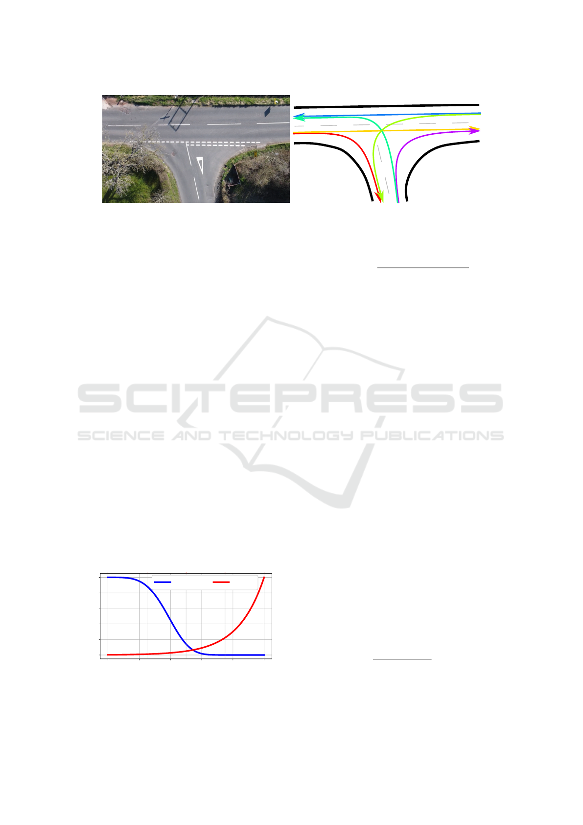
Figure 3: Visualisation of topology discretization – an intersection (left) with all possible simple paths (right).

through spline mappings, as detailed in Section 3.4:







)







+ ζ

ζ, ζ

ζ ∼ N (0

0,R

R), (12)

where µ

signiﬁes the speciﬁc path for the mappings,

and ζ

ζ represents Gaussian observation noise with zero

mean and covariance matrix R

For particle generation within the particle ﬁlter,

the estimation of the intended path µ

from global

measurements is essential. As the inverse mapping

ε has already been deﬁned, the focus is on estimating

the intended path µ

. However, this might not be de-

termined uniquely due to potential path overlaps or

shared segments, making paths indistinguishable in

certain instances. Consequently, a probability distri-

bution is employed to assess the likelihood of each

path intention. This involves combining the likeli-

hoods f

and f

of two features shown in Figure 4:

(i,µ) = e

(

−0.05D

(µ)

+1)

)

, (13)

(i,µ) = e

(

3(α

(µ)−1)

)

. (14)

The features are the distance from the closest point

projection D

(µ) = ∥p

− φ

(ε

))∥, and a dot

product α

(µ) = θ

· ψ

(ε

)) of the path heading

and measured heading of a vehicle.

0 1 2 3 4 5

(m)

0.0

0.2

0.4

0.6

0.8

1.0

likelihood (-)

−1.0 −0.5

0.0 0.5 1.0

(−)

) f

(α

)

Figure 4: Likelihood functions of features.

The combination of these likelihoods results in the

distribution over all path intentions µ:

P(i,µ) =

q(µ) f

(i,µ) f

(i,µ)

∑

j=1

q( j) f

(i, j) f

(i, j)

, (15)

where q(µ) is the overlap coefﬁcient, adjusting

the probabilities for situations involving overlapping

paths, as commonly encountered in roundabouts.

3.7 Reward Function

The reward function is a crucial component that de-

ﬁnes the behavior of the ego vehicle within the in-

tersection. It is responsible for aligning the vehicle’s

actions with our desired objectives: efﬁcient naviga-

tion through the intersection while prioritizing safety,

avoiding excessive acceleration, and preventing colli-

sions. This multi-goal task is formulated as

= r

vel

) + r

acc

) + r

crash

). (16)

The reward at each time step, denoted as r

, is com-

posed of three fundamental terms: r

vel

representing

velocity, r

acc

for acceleration, and r

crash

pertaining to

collision avoidance.

The velocity reward encourages the ego vehicle to

maintain an appropriate speed throughout its trajec-

tory. It is determined based on the deviation from the

reference velocity ∆v = v

des

− v

vel

) =

(

−R

vel

∆v if ∆v ≥ 1 ,

−R

vel

∆v

otherwise,

(17)

where R

vel

is a positive weight. The desired veloc-

ity v

des

is inﬂuenced by factors such as the curvature

) at the vehicle’s position p

along its intended

path µ

. The desired velocity is determined as:

des

= min (v

curve

lim

), (18)

where v

curve

lat,max

/κ

) is the velocity lim-

ited by the maximal acceptable lateral acceleration

lat,max

,max, and v

lim

maximal velocity limit of the

intersection.

VEHITS 2024 - 10th International Conference on Vehicle Technology and Intelligent Transport Systems

526

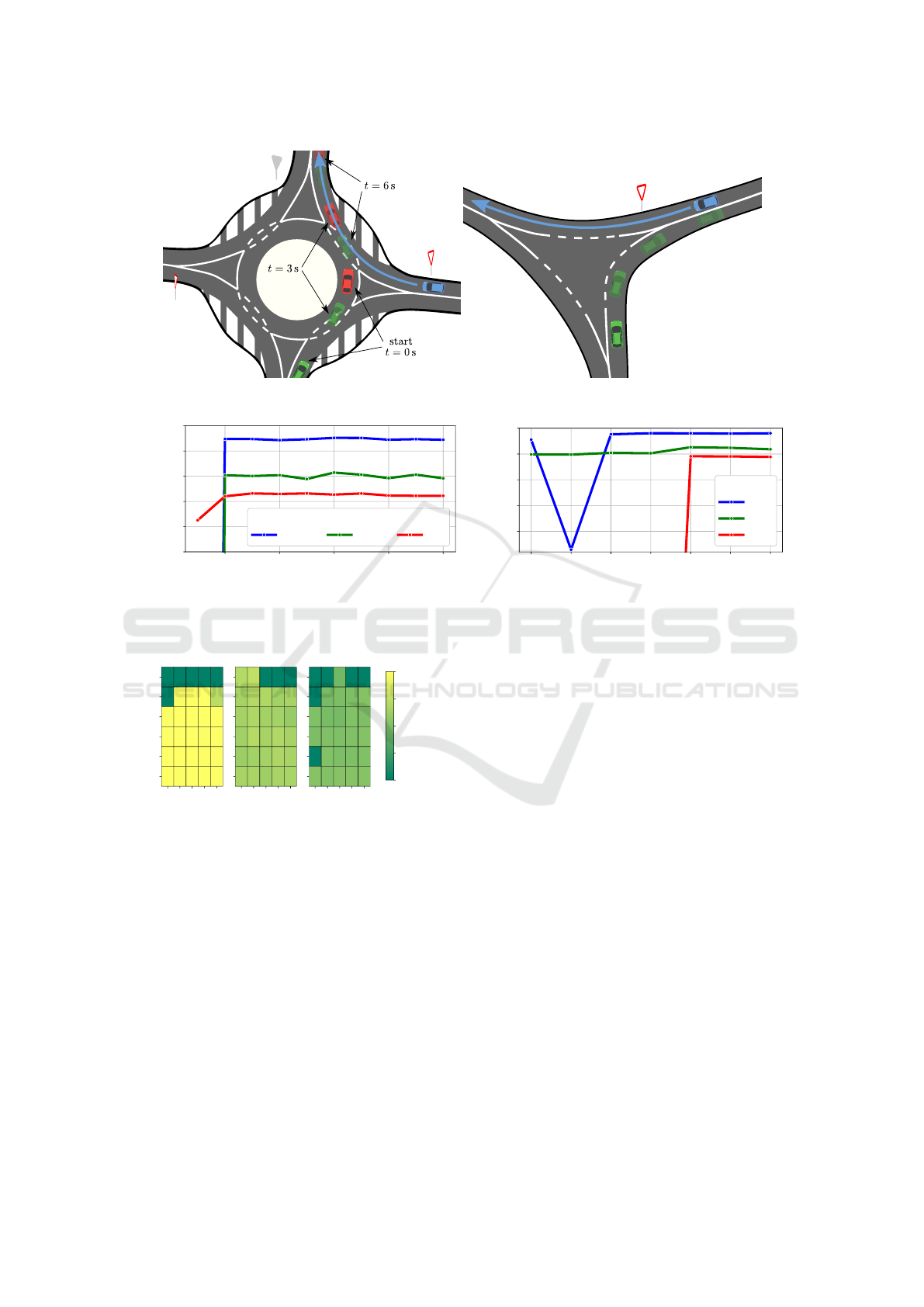
Figure 5: Simulation scenarios – roundabout (left), threeway junction (right). The ego car is represented with a blue color.

2 4 6 8 10

optimization horizon N (-)

−4000

−3800

−3600

−3400

−3200

−3000

mean nor m. reward (-)

∆t (s)

0.25 0.5 1.0

1 10 100 1000 10000 100000 1000000

UCB coeﬃcient c (-)

−5000

−4500

−4000

−3500

−3000

mean nor m. reward (-)

∆t (s)

0.25

0.5

1.0

Figure 6: Roundabout rewards – varying optimization horizon N (left), and varying UCB coefﬁcient c (right).

100

500

1000

2000

100

500

1000

2000

5000

10000

(-)

∆t = 0.25 s

100

500

1000

2000

par

(-)

∆t = 0.5 s

100

500

1000

2000

∆t = 1.0 s

−4000

−3775

−3550

−3325

−3100

mean normalized reward (-)

Figure 7: Roundabout rewards for varying n

par

and n

An acceleration penalty is imposed to prevent

abrupt changes in velocity, thus increasing driving

comfort. It is computed using a quadratic penalty

function, weighted by R

acc

≥ 0:

acc

) = −R

acc

. (19)

The collision avoidance component is designed to

prevent crashes. It assigns a negative reward −R

crash

when a collision is detected and 0 otherwise:

crash

) =

(

−R

crash

if ego crashed,

0 otherwise.

(20)

Collision detection relies on the overlap of bounding

rectangles of vehicles, as explained in Section 3.1.

4 RESULTS

In this section, we test the investigated method’s

collision-free planning capabilities and the impact of

parameter adjustments on the planning algorithm’s ef-

fectiveness. For these proposes, we ran simulations

based on data collected from aerial observations of

two speciﬁc intersections as shown in Figure 5. In

the simulations, building upon the results of (Ma

nour,

2021), we replaced a yielding vehicle with our ego

vehicle to mimic real-life situations. Even though the

use of such ofﬂine data does not include direct reac-

tions of other vehicles to the ego vehicle, we deem

it appropriate for testing situations where the ego is

expected to yield and adequately respond to the be-

havior of others. Also, our simulations assume that

the ego vehicle adheres to the point mass model (7).

We focus on the Adaptive Belief Tree (ABT) al-

gorithm’s parameters: the optimization horizon N, the

number of particles n

par

, the number of episodes n

and the Upper Conﬁdence Bound (UCB) parameter

c inﬂuencing the exploration-exploitation trade-off.

These parameters are crucial to the ABT algorithm,

and their individual impacts on the performance are

not immediately apparent. The default values of all

parameters used in our simulations are provided in

Parameter Adjustments in POMDP-Based Trajectory Planning for Unsignalized Intersections

527

2 4 6 8 10

optimization horizon N (-)

−1200

−1100

−1000

−900

−800

−700

−600

−500

−400

−300

mean norm. reward (-)

∆t ( s)

0.25 0.5 1.0

1 10 100 1000 10000 100000 1000000

UCB coeﬃcient c (-)

−1200

−1100

−1000

−900

−800

−700

−600

−500

−400

−300

mean norm. reward (-)

∆t (s)

0.25 0.5 1.0

Figure 8: Threeway rewards – varying optimization horizon N (left), and varying UCB coefﬁcient c (right).

100

500

1000

2000

100

500

1000

2000

5000

10000

(-)

∆t = 0.25 s

100

500

1000

2000

par

(-)

∆t = 0.5 s

100

500

1000

2000

∆t = 1.0 s

−1100

−975

−850

−725

−600

mean normalized re ward (-)

Figure 9: Threeway rewards for varying n

par

and n

Table 1: Default parameter values.

Description Value

A action set

{

−2,−1,0, 1

}

−2

c UCB parameter 20000

N opt. horizon 5

num. of episodes 3000

par

num. of particles 300

γ discount fact. 1

Q dyn. covariance 0

R obs. covariance diag(10

−2

,10

−2

,0)

IDM st. dev. 1 m s

−2

τ time headway 2 s

δ acc. exponent 4

min

IDM min. dist. 1 m

acc

acc. reward coef. 1

vel

vel. reward coef. 100

crash

crash reward 10000

lat,max

max. lat. acc. 0.5 ms

−2

Table 1. We obtained those values by tuning or by

following the works they were used in.

For each scenario, we tested every parameter com-

bination in 50 simulations, employing three different

time step lengths ∆t. The chosen parameter settings

signiﬁcantly inﬂuence the simulation runtime, except

for the UCB factor c, which does not alter the runtime.

To provide a clearer perspective on how these settings

impact the simulation duration, Table 2 presents a

comparison of roundabout scenario runtime estimates

Table 2: Runtime estimate with realtime percentages.

∆t (s)

Runtime (s)

default settings

Runtime (s)

= 10

, n

par

= 2 · 10

1 6 (75%) 14 (175%)

0.5 10 (125%) 42 (525%)

0.25 24 (300%) 118 (2350%)

for two distinct parameter conﬁgurations alongside

their corresponding real-time percentages. Our simu-

lation software was implemented in C++, utilizing the

TAPIR toolbox together with ROS 1, and we ran the

simulations on a laptop with an Intel i5-11500H CPU.

4.1 Roundabout Scenario

The ﬁrst scenario involves the ego vehicle approach-

ing a roundabout at 8 m s

−1

, interacting with two ve-

hicles, as seen in the left image of Figure 5. This sce-

nario tests the ability to yield and avoid crashes.

The results, depicted in Figures 6 and 7, show

the mean of normalized reward ∆t

∑

achieved for

various settings. Settings without crashes had val-

ues between −3200 and −3600. Mean reward be-

low −4000 represents occurring crashes. The reward

is also based on ∆t, as the smaller the time step, the

higher the reward because the planning algorithm has

more samples to react.

Our key ﬁndings include identifying parameter

threshold values, where their further changes have

minimal impact on performance yet signiﬁcantly in-

crease computation time. The threshold for N is 2;

since for N = 1, vehicles frequently crash at sample

times ∆t ≤ 0.5 s. For c, the threshold appears to be

10000, with regular crashes occurring at lower val-

ues, mainly for ∆t = 1 s. Crashes also happened com-

monly for n

par

≤ 100 and for n

≤ 500.

4.2 Threeway Junction Scenario

In the second scenario, the ego vehicle approaches a

three-way junction at 8 m s

−1

, while another vehicle

VEHITS 2024 - 10th International Conference on Vehicle Technology and Intelligent Transport Systems

528

with the right of way also approaches the intersection

as depicted in the right image of Figure 5. There is no

danger of crashing because the other vehicle turns in a

non-collision direction, yet this is an unknown behav-

ior initially. This scenario examines the ego vehicle’s

information-gathering capability.

Note that the reward here does not indicate the to-

tal quality of the solution; rather, it says how well the

vehicle follows the reference velocity. Slowing down

information gathering is reﬂected as a lower reward.

This is reﬂected in our results shown in Figures 8,

and 9, where parameter combinations of N, n

par

, and

that caused crashes in the roundabout scenario

yield higher rewards as they ignore the possible dan-

ger of crashing. The reference velocity is not fol-

lowed properly for the c values below the threshold,

making the rewards lower, especially for ∆t = 1 s,

and ∆t = 0.5 s. Also, the rewards for ∆t = 0.25 s

are generally lower than for ∆t = 0.5 s, indicating

that the cost of delaying a decision when more sam-

ples are available is lower relative to the total re-

ward. This behavior might be ﬁne-tuned by param-

eters R

acc

, R

crash

and R

vel

5 CONCLUSION

In this paper, we successfully veriﬁed the planning

capabilities of the investigated trajectory planning

POMDP-based method for unsignalized intersection

crossing. We executed a series of simulations based

on real-life data from aerial recordings of two distinct

intersections. The method proved capable of handling

the uncertain aspects of the problem, such as the un-

known intention of other vehicles.

Additionally, we investigated the inﬂuence of pa-

rameter adjustment on the method’s performance.

Our results indicate that there are certain well-

performing threshold values. Exceeding them yields

little to no gains and increased computation time.

This ﬁnding is beneﬁcial with regard to the future ap-

plication of this method and its derivations.

ACKNOWLEDGEMENTS

This work was co-funded by the European

Union under the project ROBOPROX (reg. no.

CZ.02.01.0100/22 0080004590) and by the Technol-

ogy Agency of the Czech Republic under the project

Certicar CK03000033.

REFERENCES

Bey, H., Sackmann, M., Lange, A., and Thielecke, J.

(2021). POMDP Planning at Roundabouts. In 2021

IEEE IV Workshops, pages 264–271.

Braziunas, D. (2003). POMDP solution methods.

Eskandarian, A., Wu, C., and Sun, C. (2021). Research Ad-

vances and Challenges of Autonomous and Connected

Ground Vehicles. IEEE Transactions on Intelligent

Transportation Systems, 22(2):683–711.

Hubmann, C., Quetschlich, N., Schulz, J., Bernhard, J., Al-

thoff, D., and Stiller, C. (2019). A POMDP Maneuver

Planner For Occlusions in Urban Scenarios. In 2019

IEEE IV, pages 2172–2179.

Hubmann, C., Schulz, J., Becker, M., Althoff, D., and

Stiller, C. (2018). Automated Driving in Uncertain

Environments: Planning With Interaction and Uncer-

tain Maneuver Prediction. IEEE Transactions on In-

telligent Vehicles, 3(1):5–17.

Klimenko, D., Song, J., and Kurniawati, H. (2014). TAPIR:

A software toolkit for approximating and adapting

POMDP solutions online. In IEEE ICRA.

Kurniawati, H. (2022). Partially Observable Markov Deci-

sion Processes and Robotics. Annual Review of Con-

trol, Robotics, and Autonomous Systems, 5(1):253–

277.

Kurniawati, H. and Yadav, V. (2016). An Online POMDP

Solver for Uncertainty Planning in Dynamic Environ-

ment. In Inaba, M. and Corke, P., editors, Robotics

Research: The 16th International Symposium ISRR,

Springer Tracts in Advanced Robotics, pages 611–

629. Springer International Publishing, Cham.

Litman, T. (2023). Autonomous Vehicle Implementation

Predictions: Implications for Transport Planning.

nour,

S. (2021). Simulation environment for testing of

planning algorithms. Master’s thesis, CTU in Prague.

Poggenhans, F., Pauls, J.-H., Janosovits, J., Orf, S., Nau-

mann, M., Kuhnt, F., and Mayr, M. (2018). Lanelet2:

A high-deﬁnition map framework for the future of au-

tomated driving. In 2018 IEEE ITSC, pages 1672–

1679.

Schulz, J., Hubmann, C., Morin, N., L

ochner, J., and

Burschka, D. (2019). Learning Interaction-Aware

Probabilistic Driver Behavior Models from Urban

Scenarios. In 2019 IEEE IV, pages 1326–1333.

Schwarting, W., Alonso-Mora, J., and Rus, D. (2018). Plan-

ning and Decision-Making for Autonomous Vehicles.

Annual Review of Control, Robotics, and Autonomous

Systems, 1(1):187–210.

Tong, W., Hussain, A., Bo, W. X., and Maharjan, S. (2019).

Artiﬁcial Intelligence for Vehicle-to-Everything: A

Survey. IEEE Access, 7:10823–10843.

Treiber, M., Hennecke, A., and Helbing, D. (2000).

Congested trafﬁc states in empirical observations

and microscopic simulations. Physical Review E,

62(2):1805–1824.

Ye, N., Somani, A., Hsu, D., and Lee, W. S. (2017).

DESPOT: Online POMDP Planning with Regular-

ization. Journal of Artiﬁcial Intelligence Research,

58:231–266.

Parameter Adjustments in POMDP-Based Trajectory Planning for Unsignalized Intersections

529