Method for Automated Parametric Studies and Evaluation Using the

Example of an Aerosol-on-Demand Jet-Printhead

Hanna Pfannenstiel, Martin Ungerer

and Ingo Sieber

Institute for Automation and Applied Informatics, KIT, Hermann-von-Helmholtz-Platz 1, 76344 Eggenstein-Leopoldshafen,

Germany

Keywords:

Computational Fluid Dynamics, Modelling, Simulation, Model Reduction, Additive Manufacturing,

Aerosol-on-Demand.

Abstract:

In this paper, we present a method for the automated determination of aerosol jet parameters for the Aerosol-

on-Demand (AoD) jet-printhead. A critical aspect in the simulation of our computational ﬂuid dynamics

(CFD) model is the simulation time due to the high model complexity in combination with a large number of

individual elements. This, together with the problem of determining the focal point through measurements on

our laboratory setup, leads to our approach of model reduction as the basis for an automated determination

of the aerosol jet parameters, which is shown using the example of determining the focal position and focal

width. Starting from a ﬂuid dynamic model, we create a reduced model by separating the variables, with

which we can predict aerosol jet parameters. The method presented here is validated by CFD simulations of

an aerosol spray with a mass of individual droplets are varied according to a Rosin-Rammler distribution.

1 INTRODUCTION

The functional printing of nanomaterials offers new

possibilities for the realization of electronic circuits

(Baby et al., 2020; Gengenbach et al., 2018; Cui,

2016; Suganuma, 2014; Choi et al., 2015), e.g. on

ﬂexible substrates and 3D components, for which

conventional lithography-based subtractive manufac-

turing processes are not suitable (IDTechEx Ltd.,

2022). The printing of functional inks also opens

up new possibilities for the realization of special

physical, optical or chemical properties (Sirringhaus

and Shimoda, 2003; Sieber et al., 2020a,b; Mag-

dassi, 2010). In general, digital printing processes

for functional printing can be categorized as Drop-

on-Demand (DoD) inkjet or aerosol jet printing pro-

cesses. The DoD inkjet printing process in particu-

lar has established itself in the additive manufacturing

of functional structures. However, it has the inher-

ent disadvantage that it requires a constant distance

between the nozzle and substrate in the range of ap-

prox. 0.3 mm to 1 mm in order to achieve high print

quality. This process requirement makes the printing

of 3D structures very complex or impossible. The

https://orcid.org/0009-0000-4026-6338

https://orcid.org/0000-0003-2811-7852

aerosol jet printing process offers an alternative for

functional printing in terms of higher resolution and

the possibility of printing on 3D structures. The basis

of this printing process is the atomization of the ink

into a ﬁne spray and the subsequent hydrodynamic

focusing by means of a sheath gas ﬂow and nozzle

geometry. The result is an aerosol jet that is colli-

mated over a range of several millimeters, i.e. the jet

width does not change in this range. This collima-

tion range makes it possible for the printed line width

to be independent of the distance between the nozzle

outlet and the substrate. This enables the aerosol jet

printing process to print on uneven surfaces and sur-

faces of any shape. The aerosol jet printing process

is currently realized as a continuous printing process

(Optomec Inc., 2024; IDS Inc., 2024), which requires

a physical interruption of the jet to print discontinu-

ous structures. A new principle for an Aerosol-on-

Demand (AoD) jet-printhead is being developed at

our institute (Ungerer et al., 2023c), which basically

enables high-frequency switching on and off of the

aerosol generation with an established sheath gas ﬂow

and thus enables on-demand printing (Sieber et al.,

2022). This is achieved by atomizing tiny amounts of

functional ink directly in the printhead. The result-

ing compact system design also enables printing in

all spatial directions and a widely adjustable distance

Pfannenstiel, H., Ungerer, M. and Sieber, I.

Method for Automated Parametric Studies and Evaluation Using the Example of an Aerosol-on-Demand Jet-Printhead.

DOI: 10.5220/0012758100003758

Paper published under CC license (CC BY-NC-ND 4.0)

In Proceedings of the 14th International Conference on Simulation and Modeling Methodologies, Technologies and Applications (SIMULTECH 2024), pages 69-79

ISBN: 978-989-758-708-5; ISSN: 2184-2841

between the nozzle and substrate (Ungerer, 2020).

Based on computational ﬂuid dynamics (CFD) simu-

lations, the design-for-manufacturing of a laboratory

setup was created and implemented (Ungerer et al.,

2022, 2023a).The CFD simulations were used to mu-

tually evaluate different nozzle geometries (Ungerer

et al., 2023b) and to determine tolerance inﬂuences in

the position of the atomizer unit. The CFD simula-

tions are very complex to calculate and require many

hours to a few days for the calculation (the CFD simu-

lations are carried out on a workstation equipped with

AMD Ryzen Threadripper 3970X processor with 32

cores, 64 threads @ 3.7GHz, 128 GB RAM, and

an Nvidia Titan RTX graphics processor with 24GB

which is available at our institute. In order to allow

other processes to still take place on the workstation,

only 28 cores are utilized in the simulations of this

paper.). In addition, when measuring the aerosol jet

on the test setup, we realized that it is not possible to

determine the jet width and the location of the focus

position with our measurement equipment.

The contribution that we address in this paper is

the automated determination of the focal position as

a function of the droplet mass or its emission angle

during aerosol generation on the basis of predictions

made using a reduced model. The model reduction

procedure is based on the separation of the mass and

emission angle variables.

This paper is organized as follows: Section 2 de-

scribes the laboratory setup of the AoD printhead,

Section 3 presents the CFD model and motivates the

model reduction, which is used to determine the fo-

cal position of the droplets. Section 4 is dedicated

to analyzing the derived method in comparison with

the simulation of an aerosol spray with a mass dis-

tribution described by a Rosin-Rammler distribution.

Section 5 deals with the discussion of the results and

section 6 will close the paper with conclusions.

2 THE AoD SETUP

The AoD jet-printhead is shown schematically in Fig-

ure 1 and comprises an atomizer unit that generates

the aerosol on demand and directly inside the print-

head, an antechamber with four inlets for the sheath

gas equidistantly distributed around the circumfer-

ence of the printhead, a mixing chamber and a noz-

zle. The antechamber is designed to ensure a ho-

mogeneous annular sheath gas ﬂow inside the mix-

ing chamber of the printhead where the aerosol is

ejected from the atomizer unit and to directly focus

the aerosol in combination with the inner contour of

the mixing chamber and the nozzle. The nozzle of the

printhead is manufactured in two parts (Ungerer et al.,

2023a).

Figure 1: Schematic of the AoD jet-printhead.

The fabricated laboratory prototype of the devel-

oped AoD jet-printhead is integrated into a labora-

tory test setup in order to characterize the generated

aerosol jet after the nozzle exit (Sieber et al., 2022).

The laboratory test setup, consisting of an ink sup-

ply, a sheath gas supply, the printhead with a func-

tion generator and an optical observation equipment,

is schematically depicted in Figure 2.

The ink supply comprises an ink reservoir, a time-

pressure dispenser that is used as open-loop control of

the pressure inside the ink reservoir and a mobile air

compressor acting as compressed air supply for the

dispenser. The sheath gas supply is composed of an

Argon gas cylinder with a pressure regulator, a mass

ﬂow controller and manifolds. The ink supply is con-

nected to the atomizer unit of the printhead. The actu-

ator of the atomizer unit is connected to the frequency

generator. Water is used as test ﬂuid. The sheath gas

supply is connected to the four inlets of the antecham-

ber of the printhead. The aerosol jet after nozzle exit

is studied by means of a Keyence VHX-7020 digital

camera with a Keyence VH-Z20R microscope zoom

lens and a 20 W Tapfer 5004LTF LED light, inclined

by 45

◦

to the camera’s optical axis.

Figure 3 shows images of the aerosol jet after the

nozzle exit. As can be seen from Figure 3 a), the

aerosol jet is collimated over a length of about 60 mm

after the nozzle exit. Images taken with higher mag-

niﬁcation (Figures 3 b) and c)) reveal that it is al-

most impossible to precisely measure the real diam-

eter of the aerosol jet and to determine the focal point

with the presented setup, in particular, as individual

droplets outside the actual, clearly visible beam are

hardly to be detected.

SIMULTECH 2024 - 14th International Conference on Simulation and Modeling Methodologies, Technologies and Applications

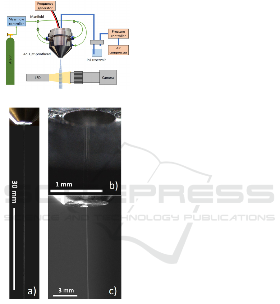
Figure 2: Schematic of the optimized laboratory setup.

Figure 3: Microscope images showing a) the collimation

length, b) the nozzle oriﬁce and c) the focused aerosol jet at

planned working distance after nozzle exit ).

3 MODELING

3.1 The CFD Model

As previously mentioned the AoD Printer is a use case

that is very difﬁcult to do physical measurements on.

Therefore a Computer Fluid Dynamics (CFD) model

has been created to gain more information about the

ﬂow regime that is important to the functionality of

the device. CFD is an established technology which

calculates ﬂow regimes based on the Navier-Stokes

equations. The CFD software used in this paper is An-

sys Fluent 2023 R2. In most situations a Direct Nu-

merical Simulation (DNS) through the Navier-Stokes

equations is too computationally expensive if turbu-

lence phenomena on a multitude of scales should

be represented. Therefor averaging terms and tur-

bulence models are necessary to simulate the phe-

nomena. For computationally economic reasons the

Reynolds-Averaged Navier-Stokes (RANS) in combi-

nation with the k-ω-SST turbulence model was cho-

sen as they provide the required accuracy for most en-

gineering applications while not increasing the com-

putational time signiﬁcantly (Sieber et al., 2022). In-

terested readers can ﬁnd more detailed information

about the RANS and k-ω models in Wilcox (2006)

and Menter (1994).

The CFD model features the geometry of the

printhead starting at the inlet channels to the homoge-

nization chamber as well as an area that spans 26 mm

past the nozzle exit to simulate the free jet.

The mesh in CFD simulations greatly inﬂuences

the quality of the result. Areas with high gradients

need a ﬁne mesh for the gradients to not get lost in

the averaging over an element. Additionally, struc-

tured meshes which are aligned with the direction of

the ﬂow improve numerical diffusion (Ungerer et al.,

2022). Unstructured meshes on the other hand offer a

simpler meshing process and they require less control

to ensure that they are set up properly. As the area

of the free jet is of great interest a structured, hexa-

hedral mesh will be used. The mesh of the free jet

features elements with smaller length near the noz-

zle exit and longer cells towards the end as can be

seen in Figure 5. Inside the printhead the center is

meshed structurally with ﬁner cell resolution. In the

mixing chamber an unstructured tetrahedral mesh is

generated as the ﬂow in those domains is less impor-

tant and computational resources can be saved. The

generated mesh for the inside of the printhead can be

seen in Figure 4.

As the Euler-Lagrange model used to track the

discrete phase involves particles the cell size must be

large enough for a particle to be entirely contained

in a single cell. Ungerer et al. (2023a) measured a

droplet size of up to 20 µm at the capillary exit. A

previous independence study dealt with the level of

detail in the mesh and found a mesh with 2.1 million

elements to be sufﬁciently accurate with any increase

in the mesh precision not necessarily resulting in a

Method for Automated Parametric Studies and Evaluation Using the Example of an Aerosol-on-Demand Jet-Printhead

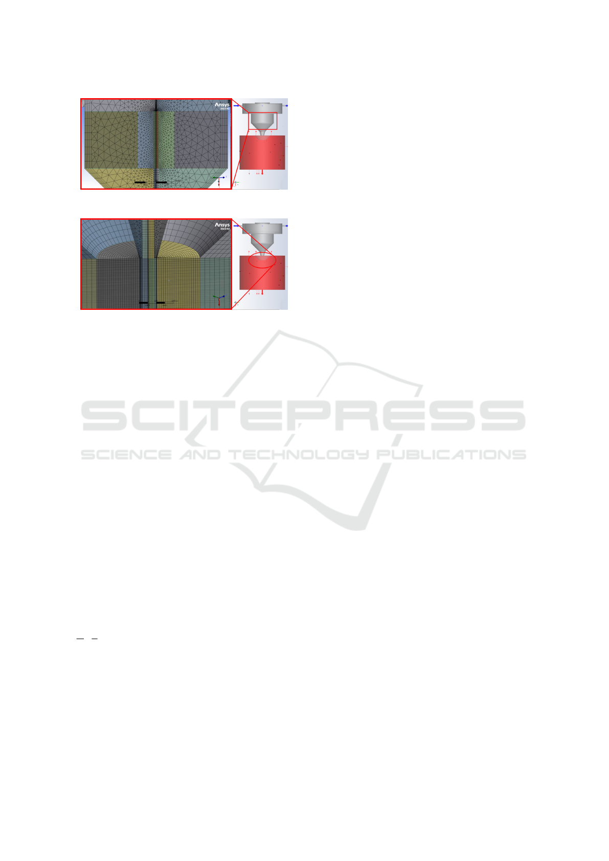
Figure 4: The mesh of the mixing chamber.

Figure 5: The mesh at the beginning of the free jet area.

worthwhile trade-off of improved accuracy over cal-

culation time (Ungerer et al., 2023d). The minimum

element size in this mesh is 33 µm which fulﬁlls the

condition set by tracking of the discrete phase.

As it is the ﬁnal goal, a stationary solution is eval-

uated in the CFD simulation where the sheath gas has

a fully developed ﬂow. From that follows the assump-

tion that the entire printhead is completely ﬁlled with

the sheath gas Argon while the free jet area is predom-

inantly air. While gases have similar densities and

viscosities in absolute terms comparing their material

properties relatively shows a bigger difference. In or-

der to properly model the interaction in the free jet as

the two gases mix a multiphase model is utilized. An-

sys provides multiple multiphase models that vary in

their use case and complexity. For this application the

Volume-of-Fluid (VoF) model is chosen. It introduces

the volume fraction as an additional variable to solve

for each cell in the continuous equations. The volume

fraction is calculated according to Equation 1 (AN-

SYS, Inc., 2023a) where q is the index of the phase,

˙m

is the mass transport between phases and S

is a

user-deﬁnable mass source. In our model we use its

default value zero.

∂

∂t

(α

) + ∇ · (α

⃗v

) = S

∑

p=1

( ˙m

− ˙m

)

(1)

All other material properties such as viscosity and

density are derived by linear blending of the values of

each individual material through its volume fraction.

The interfacial areas of the phases are afterwards re-

constructed from the volume fractions. As air and ar-

gon don’t form a sharp interface a dispersed modeling

was chosen to reﬂect the area of mixture.

3.2 Determining the Focal Point

The focal point of the aerosol jet is the cross section

in which the aerosol covers the smallest area. The

coordinate system used throughout this paper can be

seen in Figure 1: Cylindrical coordinates are used due

to rotation symmetry. The origin is at the nozzle exit

of the printhead and the x-Axis is the direction of the

free jet. r is the radial direction and φ the azimuthal

angle. In order to determine the position of the fo-

cal point, the particle tracks from the CFD are ex-

ported. These records feature the position of each par-

ticle throughout all simulated timesteps. The resulting

dataset can then be scanned through step by step and

the r-position of each particle can be calculated. Be-

cause there are a thousand particles distributed in all

azimuthal angles and due to rotational symmetry of

the geometry it is assumed that the coordinate φ is of

no relevance to the jet and that it is sufﬁciently round

along its entire travel distance. Therefore, determin-

ing the radial distance r to the center axis is sufﬁcient

to determine the size of the aerosol jet.

While scanning through the dataset the size of the

aerosol jet in each cross section is imposed by the par-

ticle that is furthest away from the x-Axis. Stray par-

ticles cause overspray on the substrate which leads to

undeﬁned boundaries in the print image and can have

serious effects on the function. Therefor it is impor-

tant to consider outliers when determining where the

focal point lies. When the focal point is found it can

be described by its x-position x

Focal

, which will be

called the focal point position throughout this paper,

and the r-position of the most outward particle in the

focal plane r

Focal

which is called the Focal Spot Half

Width (FSHW) throughout this paper.

3.3 Automatic Parameterization

As the atomizer unit is what sets the AoD printing

method apart from other technologies, as mentioned

in Section 1, its development is of great importance.

While the sheath gas in combination with the nozzle

geometry has the biggest inﬂuence on the focusing of

the aerosol spray, its ﬂow is assumed to be station-

ary under operating conditions. The biggest remain-

ing inﬂuence on the position of the focal point of the

aerosol spray lies in the atomization of the ink and

what the initial attributes of the individual droplets

are when they enter the mixing chamber. Relevant

attributes are the mass and direction of travel of a par-

ticle. Therefore, a study of what values are advanta-

geous is highly desirable as it can be used to guide

further development of the atomization unit.

For this purpose, a parametric study of the parti-

SIMULTECH 2024 - 14th International Conference on Simulation and Modeling Methodologies, Technologies and Applications

cle’s mass m and angle of injection θ is made. The

injection angle was chosen as it describes the direc-

tion of travel of the particles in the cone injection

model of Ansys Fluent. More detail about the def-

inition of the cone injection model can be found in

ANSYS, Inc. (2023b). The decision is made to in-

corporate Kadi4Mat v0.45.3 (Brandt et al., 2021), an

electronic lab notebook (ELN), into the process in or-

der to easily store data in a uniform and code accessi-

ble way. The boundaries for the parametric study are

taken from previous studies (Ungerer et al., 2023a).

The particle size and therefor mass is varied from

1.05 × 10

−5

m to 1.85 × 10

−5

m radius with a step

size of 0.05 × 10

−5

m. The injected droplets are set

to be liquid water at a temperature of 300 K and since

there is no active heating or cooling present, the den-

sity of the water doesn’t change signiﬁcantly and the

droplet size correlates directly with the droplet mass.

The injection angle θ is varied from 0

◦

to 45

◦

in 5

◦

steps. The result is a set of 17 simulations with vary-

ing mass at a constant injection angle of 35

◦

and a

second set of ten simulations with a varying injection

angle at a constant mass of 1.2859 ng which results

from a particle radius of 1.35 × 10

−5

Fluent allows for the continuation of previously

simulated cases. Because the aerosol is simulated

through a Lagrange-Euler model it doesn’t affect the

ﬂow of the continuous phases. This allows the simu-

lation of one case until the sheath gas ﬂow has fully

developed. Once convergence is reached in that case

it is saved as a base case. In order to save on computa-

tion time all simulations will use the fully developed

ﬂow from the base case as a starting point by loading

the case data from the base case, modifying the injec-

tion parameters and continuing the simulation. Due

to the different injection parameters the residuals will

spike and the simulation is run until they are back be-

low the boundaries for convergence.

Each simulation gets its own record in Kadi4Mat

which features all of the data that differs from the

base case which is linked in the record as well. A

script is written in Python 3.11.3 which loads the

base case into Fluent via the Kadi apy v.0.35.0 and

ansys-ﬂuent-core v.0.18.2 Libraries. Afterwards the

code modiﬁes the relevant parameters speciﬁed in the

ELN records and starts the simulation with the modi-

ﬁed parameters. After the simulation has ﬁnished, the

Python code saves the ﬁnished simulation data back

into its corresponding record where it can be accessed

for evaluation.

For the evaluation MATLAB 2023b is used. As

the inﬂuence of the initial condition on the focal point

of the individual particle is of interest, the focal point

needs to be evaluated for each individual particle as

well. The method is equivalent to the method de-

scribed in Section 3.2. The result is a set of 1000 focal

points with their corresponding initial conditions.

The relationship between the initial conditions and

the focal point is complex. In order to gain simpliﬁed

correlations a model reduction is attempted through

the parametric study and a mathematical model needs

to be selected. For this example, it is assumed that

the mass and injection angle do not affect each other

and that their inﬂuences on the focal point are inde-

pendent. They can then be separated mathematically

into the individual inﬂuence functions F

which de-

scribes the inﬂuence that the variable q has on the

variable p. These functions are determined by ex-

amining the change of the focal point position and

FSHW throughout the simulations where the initial

conditions m and θ of the particles are modiﬁed. In

each of the previously mentioned two sets of simula-

tions only one initial condition is modiﬁed while the

other remains the same. By plotting the focal point

position and FSHW over the initial condition their re-

lation can be displayed. The inﬂuence functions F

are determined by ﬁtting a regression curve to the re-

sults.

Because each inﬂuence function describes the ab-

solute position and half width of the focal point

adding them together results in the doubling of both

values. In order to negate that effect a ﬁxed offset

value is added to the inﬂuence function. Equations 2

and 3 show the ﬁnal equations to determine the focal

point position and FSHW of a particle based on its

initial conditions in a fully developed sheath gas ﬂow.

Focal

(m,θ) = F

(m) + F

xθ

(θ) + x

o f f set

(2)

Focal

(m,θ) = F

(m) + F

rθ

(θ) + r

o f f set

(3)

4 PARAMETRIC STUDY

4.1 Determining the Focal Point

When exporting the particle tracks, every particle

is listed with all of its positions and mass at every

timestep it is simulated. Naturally not all particles

share the same x-coordinate in the same row of the

export ﬁle. Therefor the MATLAB code scans the

ﬁle row by row and looks for previously speciﬁed

x-positions of a particle. If the speciﬁed x-position

lies between two x-positions from the exported ﬁle,

all variables are interpolated linearly. The result is a

dataset with synchronized data of all particles at spe-

ciﬁc cross sections. The cross sections were evaluated

in intervals of 0.1 mm starting at the nozzle exit. For

Method for Automated Parametric Studies and Evaluation Using the Example of an Aerosol-on-Demand Jet-Printhead

each cross section the r-position and mass of each par-

ticle is saved in a text ﬁle.

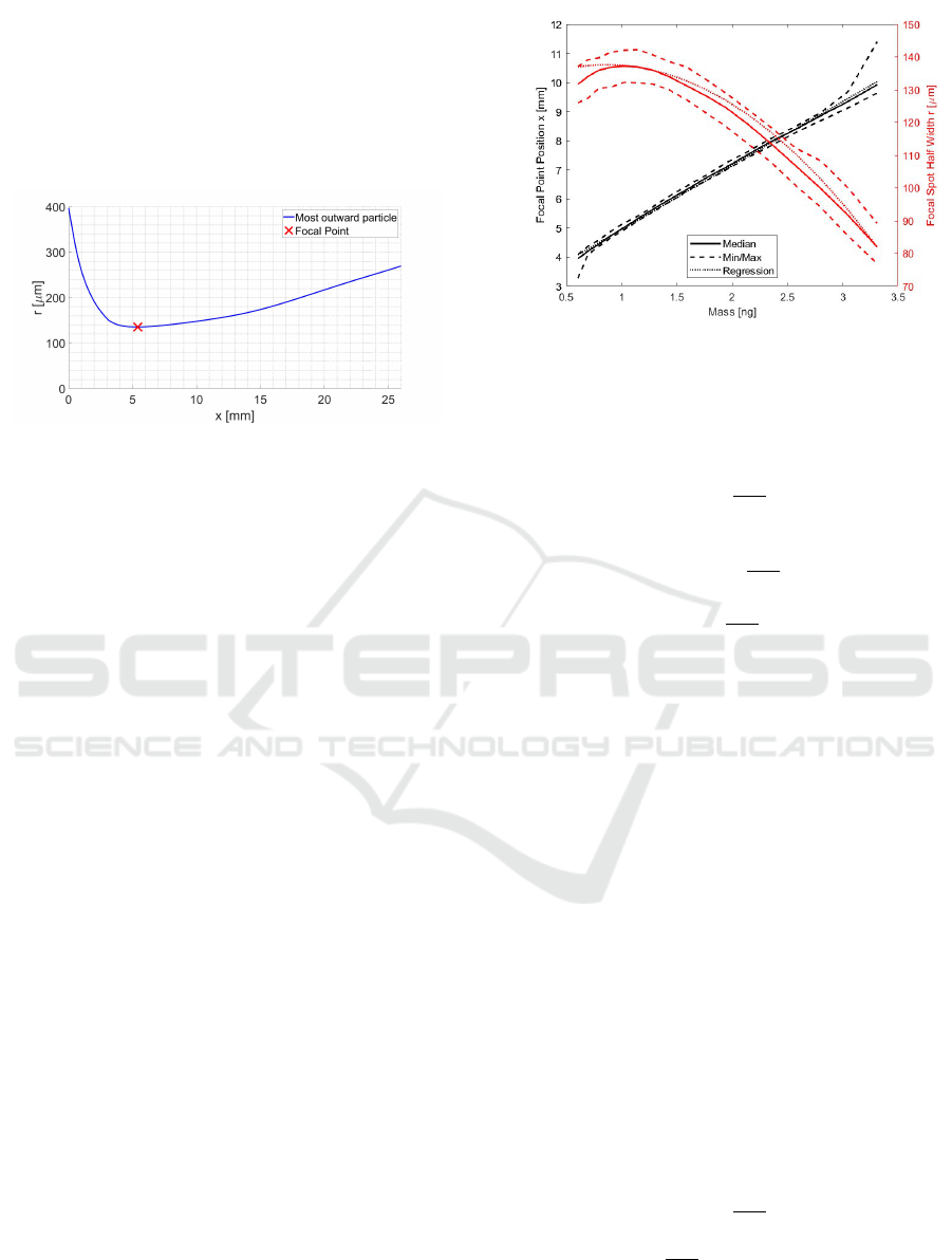
In a second step all of the cross sections can be

evaluated as described in Section 3.2. The result is

displayed in Figure 6 where the half width of the

aerosol jet is plotted over the distance from the nozzle

exit. The focal point is marked as well.

Figure 6: Half width of the aerosol jet after exiting the noz-

zle.

The accuracy of the focal point depends on the

distance between slices that are evaluated. The plot-

ted values in Figure 6 belong to a simulation with a

Rosin-Rammler mass distribution and a random injec-

tion angle up to 45

◦

for each particle. The simulation

will be discussed later in more detail.

4.2 Model Reduction

As described in Section 3.3 a parametric study with

varying mass and injection angle is simulated to de-

termine whether these have a signiﬁcant inﬂuence on

the focal point. The initial parameters in the simu-

lations are tightly controlled and random variance is

suppressed. The focal point position of each individ-

ual particle, i.e. the point of each individual particle

with the closest distance to the central axis, as well

as the FSHW can be determined in an analogue way

as the entire jet. After determining these parameters

for each particle in one simulation, the median, min-

imum and maximum values are determined and plot-

ted over the varied parameter. For the mass variance

these graphs are shown in Figure 7.

The solid line represents the median and the

dashed lines the minimum and maximum value re-

spectively. The small span of the data for each mass

indicates that the inﬂuence of the particle mass domi-

nates the position and half width of the focal point if

the injection angle is kept constant. In addition, the

graph shows a linear effect of particle mass on the

focal point position with a more massive particle in-

creasing the x-position, which is desirable. The effect

of the particle mass on the FSHW seems quadratic

within the observed boundaries. A more massive par-

Figure 7: The inﬂuence of the particle mass on the focal

point position and FSHW.

ticle also resulting in a smaller half width is also de-

sirable. For both curves their respective regression

functions were determined to:

(m) = 2.1996 × 10

· m + 2.747 mm (4)

(m) = −9.2749 × 10

· m

+ 1.597 × 10

· m + 0.1288 mm (5)

The regression functions are plotted in Figure 7 as the

dotted line. The coefﬁcient of determination for the

regression curves are R

= 99.6% and R

= 97.7%

For the inﬂuence of the injection angle the graph

shows a similarly small span of the datasets. As can

be seen in Figure 8 the injection angle has no effect on

the focal point position. The zero-degree simulation

is a special case which represents an injection where

all particles are injected in a line oriented along the

x-axis. Naturally, this results in a much smaller size

and it moves the focal point very close to the nozzle

exit as the particle tracks will widen in the free jet

due to turbulence effects. Hence, the inﬂuence of the

zero-degree simulation is neglected for determining

the focal point position.

The inﬂuence of the injection angles on the FSHW

seems to follow an exponential curve. For simplic-

ity and linearity, the regression ﬁt was made with a

quadratic function. The resulting regression functions

are:

xθ

(θ) = 0 (6)

rθ

(θ) = −3.915 × 10

−5

◦

· θ

+ 3.9603 × 10

−3

◦

· θ + 4.5856 × 10

−2

mm (7)

The corresponding coefﬁcient of determination is

rθ

= 99.3%. Each of the inﬂuence functions besides

SIMULTECH 2024 - 14th International Conference on Simulation and Modeling Methodologies, Technologies and Applications

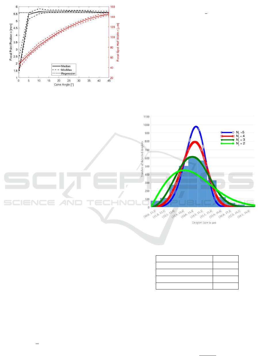
Figure 8: The inﬂuence of the injection angle on the focal

point position and FSHW.

xθ

describes the absolute value of the position or half

width of the focal point. As the individual inﬂuence

equations are added together according to Equations

2 and 3 the results are too large as the absolute po-

sition and half width is evaluated twice. An offset is

necessary to correct the functions. Since F

xθ

= 0 there

is no need for an offset to the x-Position and F

fully

describes the focal point position. For the FSHW the

point:

Focal

(1.2859ng,35

◦

) = 135.94 µm (8)

is chosen as a boundary condition as the two sets

of simulation share one simulation with these initial

parameters. r

o f f set

is determined through the bound-

ary condition and the resulting functions for x

Focal

and

Focal

are:

Focal

(m) = F

(m) (9)

Focal

(m,θ) = F

(m) + F

rθ

(θ) − 0.134 57mm (10)

4.3 Validation of the Reduced Model

As the testbed at our institute is currently inoperable,

a theoretical approach for validation is chosen. In or-

der to validate the determined inﬂuence functions a

simulation using a random distribution for the parti-

cle parameters is simulated. The injection angle θ

is randomized by using a solid cone as the injection

model (Ungerer et al., 2023d). The size, and hence

the mass of the droplets, has previously been mea-

sured by Walter (2022) and the results are shown in

Figure 9. In order to emulate the measurements in

the simulation environment, a distribution curve is ﬁt-

ted to the results. A commonly used distribution for

particle size is the Rosin-Rammler distribution (AN-

SYS, Inc., 2023b). The distribution revolves around a

mean diameter d of the droplets and a spread parame-

ter N

in order to calculate the mass fraction Y

of all

droplets that have a diameter greater than d:

= e

−(d/d)

(11)

Ansys Fluent offers the distribution by assigning each

particle one of several distinct sizes. The user can

enter the minimum, maximum and mean size, spread

parameter N

as well as how many distinct sizes An-

sys should deﬁne. The displayed droplet sizes match

the boundaries introduced in Section 3.3 and therefor

result in the same masses as examined throughout this

paper spanning approximately 0.6 ng to 3.3 ng. The

resulting inputs for Fluent are listed in Table 1. The

number of diameters determines how many evenly

spaced, discrete masses Fluent can assign to the par-

ticles. Ten was chosen to reﬂect the ten measured in-

tervals from Figure 9.

Figure 9: Histogram of measured droplet sizes with various

Rosin-Rammler distributions (Walter, 2022).

Table 1: The Rosin-Rammler Size Distribution values.

Minimum Radius 10.5 µm

Mean Radius 13.9 µm

Maximum Radius 18.5 µm

Spread Parameter N

Number of Diameters 10

The mass of each particle can be read from the ex-

port of the particle tracks. The injection angle of each

particle is determined by observing the cross section

of the aerosol 0.1 mm away from the capillary. It is

assumed that the sheath gas has no major inﬂuence on

the position of the particles near their injection point.

The injection angle for each particle is then calculated

by taking the arctangent:

θ = atan



0.1mm



(12)

Method for Automated Parametric Studies and Evaluation Using the Example of an Aerosol-on-Demand Jet-Printhead

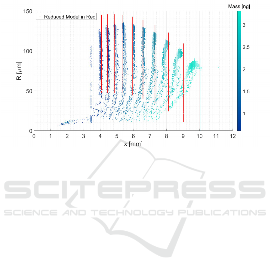
Figure 10: The focal point position and half width of each particle from the Rosin-Rammler simulation as well as from the

reduced model. The focal points belonging to the Rosin-Rammler simulation are colored by the particle mass. The estimated

focal points by the reduced model are displayed in red.

Using the initial conditions m and θ and Equa-

tions 9 and 10 the assumed focal point position and

FSHW for each particle is calculated. The actual po-

sition and half width of the focal points is determined

as described in Section 3.3.

Figure 10 shows the calculated focal point posi-

tions (shown in red) and those simulated with the

Rosin-Rammler distribution (colored by the particle

mass). The focal points are sorted into ten easily dis-

tinguishable groups depending on their mass. For big-

ger masses, the focal point position increases. For

particle masses smaller than 2.5 ng there is good

agreement between the prediction and the simulation.

Looking at the injection angles, it can also be ob-

served that particles with a larger injection angle have

a larger focal length. The corresponding graph can be

found in the Appendix.

5 RESULTS AND DISCUSSION

The results of the Rosin-Rammler simulation which

are shown in Figure 10 make it apparent that there

are effects that have not been captured by the reduced

model. The results from Section 4.2 predict that the

injection angle has no effect on the focal point posi-

tion. This is largely true for the groups of particles

with a lower mass. Their columns on the left side in

Figure 10 are mostly vertical whereas the columns of

particles with more mass to the right are slanted. This

means that for particles with a higher mass, the injec-

tion angle starts affecting the Focal Point Position or

a third, not previously evaluated, effect plays a role.

This has not been captured by the parametric study.

In order to combat this discrepancy, more parameter

combinations can be simulated. If computing time is

of concern the main simulations to determine a model

can be handled as shown in this paper. But in addition,

random sample simulations can be scattered through

the boundaries of the initial parameters to validate the

determined model. The effect that for more massive

particles the injection angle gains inﬂuence on the fo-

cal point position could have been observed in this

case and the independent model reduction could have

been discarded or extended sooner.

As no reduced model is perfect there is a need to

determine a validity domain. The validation criteria

depend on the context but for this example an allowed

relative error of the reduced model compared to the

Rosin-Rammler simulation is chosen. For the focal

point position a relative error of 5% in either direc-

tion is considered acceptable. For the FSHW a rela-

tive error of 5% was deemed acceptable if the reduced

model predicts a larger half width. But as overspray

is an issue for the AoD printing process, no error is

tolerated if the reduced model predicts a smaller half

width than the resulting simulation. The relative er-

rors in both dimensions are calculated for all particles

SIMULTECH 2024 - 14th International Conference on Simulation and Modeling Methodologies, Technologies and Applications

and plotted over their initial parameters. The plots can

be seen in Figures 11 and 12.

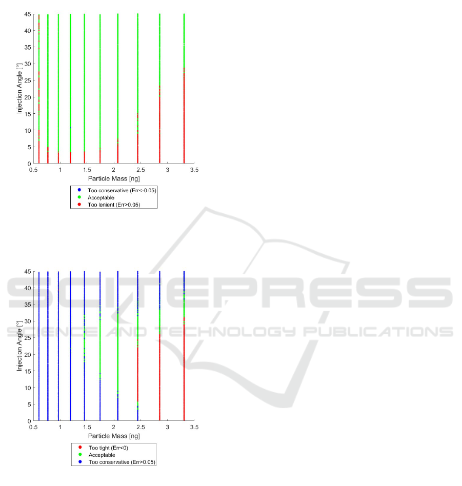
Figure 11: The relative error of the focal point position

when comparing the reduced model to the Rosin-Rammler

simulation colored by acceptance.

Figure 12: The relative error of the FSHW when comparing

the reduced model to the Rosin-Rammler simulation col-

ored by acceptance.

The focal point position is described well for

larger injection angles. Towards 0

◦

the deviation be-

comes too large as the focal point shifts closer to the

nozzle as described earlier in this section. The FSHW

has a low validity domain under the selected toler-

ances. For most initial conditions the estimate by the

reduced model is too conservative and the FSHW is

predicted too big. This is not necessarily harmful for

the AoD process as the aerosol jet will be smaller

than the reduced model describes. However, the er-

ror quickly becomes too large. Additionally, towards

the more massive particles the estimate becomes too

tight. This likely results out of the dependence of

the two initial parameters which is not considered by

the reduced model yet seen by the slantedness of the

more massive particle groups in Figure 10. The result

is that the two inﬂuence functions F

and F

rθ

both

go towards a negative direction when approaching big

masses and small injection angles respectively. These

two inﬂuences added together even result in negative

FSHWs at the extreme cases. Clearly the reduced

model offers only limited validity around 1.85 ng and

◦

for determining the FSHW.

From this point there are multiple options: Bound-

aries in which the reduced model is limited can be

determined and saved in an ELN. If any future simu-

lations fall into those boundaries the reduced model

can be taken advantage of in order to reduce com-

putation time in the future. If the reduced model is

not deemed accurate enough a different mathematical

model can be assumed and evaluated in order to deter-

mine the best model reduction. Additionally, the re-

duced model can be discarded but the general trends

can be used. In this example it was discovered that

bigger particles and smaller injection angles are fa-

vorable to reduce the FSHW in the free jet. This in-

formation can be kept in mind when developing the

atomizer unit. What path is the most sensible depends

on the application that this method is adapted to.

6 CONCLUSIONS AND

OUTLOOK

A method for an automated parametric study through

the example of an AoD jet-printhead has been debated

in this paper. The method contains an organized data

storage through the use of the ELN Kadi4Mat. All

steps described in Sections 3 and 4 of this paper can

be done by scripts and application programming in-

terfaces (APIs) of relevant software.

The method has been applied successfully to have

the computer semi-autonomously determine a re-

duced model of a ﬂow phenomena. While the model

reduction made in this paper did not prove accurate

enough to describe the focal point of a particle loaded

stationary ﬂow outside of a speciﬁed domain, that was

not the main intention of this paper. It was merely

a simple example of the proposed method in action.

In a greater context than this paper would support,

more sophisticated models can be used as a basis for

the model reduction and comparisons between differ-

Method for Automated Parametric Studies and Evaluation Using the Example of an Aerosol-on-Demand Jet-Printhead

ent models could be made to determine the best. If

paired with physical tests, model parameters can be

changed in the CFD software and the resulting ﬂow

can be compared to real observation in order to deter-

mine which model parameters reﬂect reality the best.

This possibility is the basis of a digital twin that is

currently being developed at KIT. The digital twin

is supposed to accompany the AoD printing proce-

dure featured in this paper. The AoD printhead repre-

sents a complex problem with many interactions that

are not sufﬁciently describable by established theo-

ries. The method presented in this paper can help to

develop empirical models in a semi-automated way.

While human supervision is still necessary, the work-

load is greatly reduced. Another possibility is that a

human can root the automatically generated empiri-

cal models through established theory and push the

understanding of the corresponding ﬁeld forwards.

Another possibility for this method is the model

reduction. Only one simple type of mathematical

model has been examined in this paper. However, it

is possible to try several different mathematical model

reductions of complex problems and see which reduc-

tion does the best at emulating the complex interac-

tion. This would result in computationally cheaper

correlations which lessens the calculational load of a

digital twin.

The main advantage of this method is the adapt-

ability. The ELN provides a good structure for or-

derly and automated data storage. As long as the

simulation software of interest supports scripted pro-

cesses through an API, the procedure can be adapted.

The setup of this method is labor-intensive based on

the scope of what it is adapted to as all options for

parametrization need to be coded in. This effort is

also heavily dependent on the quality and ﬂexibility

of the API of the simulation program. This makes it

suitable for larger or long-term applications such as a

digital twin where the overhead cost of programming

is smaller compared to the work that is saved through-

out the lifespan of the model.

ACKNOWLEDGEMENTS

The mesh independence study as well as the deter-

mining of the Rosin Rammler distribution values were

done by Tim Walter who we thank for his contribu-

tions.

The authors conﬁrm that no artiﬁcial intelligence

(AI) was used in generating the text of this article.

REFERENCES

ANSYS, Inc. (2023a). Ansys Fluent Theory Guide. AN-

SYS, Inc., release 2023 r1 edition.

ANSYS, Inc. (2023b). Ansys Fluent User’s Guide. ANSYS,

Inc., release 2023 r1 edition.

Baby, T. T., Marques, G. C., Neuper, F., Singaraju, S. A.,

Garlapati, S., von Seggern, F., Kruk, R., Dasgupta, S.,

Sykora, B., Breitung, B., Sukkurji, P. A., Bog, U., Ku-

mar, R., Fuchs, H., Reinheimer, T., Mikolajek, M.,

Binder, J. R., Hirtz, M., Ungerer, M., Koker, L., Gen-

genbach, U., Mishra, N., Gruber, P., Tahoori, M., Hag-

mann, J. A., von Seggern, H., and Hahn, H. (2020). Print-

ing technologies for integration of electronic devices and

sensors. In Sidorenko, A. and Hahn, H., editors, Func-

tional Nanostructures and Sensors for CBRN Defence

and Environmental Safety and Security, NATO Science

for Peace and Security Series C: Environmental Security,

pages 1–34. Springer Netherlands, Dordrecht.

Brandt, N., Griem, L., Herrmann, C., Schoof, E.,

Tosato, G., Zhao, Y., Zschumme, P., and Selzer,

M. (2021). Kadi4mat: A research data infrastruc-

ture for materials science. Data Science Journal,

20:8. https://datascience.codata.org/articles/10.5334/dsj-

2021-008.

Choi, H. W., Zhou, T., Singh, M., and Jabbour, G. E. (2015).

Recent developments and directions in printed nanoma-

terials. Nanoscale, 7(8):3338–3355.

Cui, Z., editor (2016). Printed electronics: Materials, tech-

nologies and applications. John Wiley & Sons, Higher

Education Press, Singapore, 1st edition.

Gengenbach, U., Ungerer, M., Aytac, E., Koker, L., Re-

ichert, K.-M., Stiller, P., and Hagenmeyer, V. (2018).

An integrated workﬂow to automatically fabricate ﬂexi-

ble electronics by functional printing and smt component

mounting. In Vogel-Heuser, B. and Lennartson, B., ed-

itors, Proc. 14th IEEE International Conference on Au-

tomation Science and Engineering (CASE), pages 1624–

1629.

IDS Inc. (2024). Nanojet aerosol print technology. https:

//www.idsnm.com/. Last accessed on Feb. 12, 2024.

IDTechEx Ltd. (2022). 3d electronics/additive electron-

ics 2022-2032: 3d printed electronics, molded intercon-

nect devices, in-mold electronics, aerosol jet, 3d metal-

lization, laser direct structuring, additively manufactured

electronics. sample pages. https://www.idtechex.com/e

n/research-report/3d-electronics-additive-electronics-2

022-2032/860. Last accessed on Feb. 12, 2024.

Magdassi, S., editor (2010). The chemistry of inkjet inks.

World Scientiﬁc Publishing, Singapore.

Menter, F. R. (1994). Two-equation eddy-ciscosity turbu-

lence models for engineering applications. AIAA Jour-

nal, 32(8):1598–1605.

Optomec Inc. (2024). Aerosol jet technology. https://opto

mec.com/printed-electronics/aerosol-jet-technology/.

Last accessed on Feb. 12, 2024.

Sieber, I., Thelen, R., and Gengenbach, U. (2020a). Assess-

ment of high-resolution 3d printed optics for the use case

of rotation optics. Optics express, 28(9):13423–13431.

Sieber, I., Thelen, R., and Gengenbach, U. (2020b). En-

hancement of high-resolution 3d inkjet-printing of op-

SIMULTECH 2024 - 14th International Conference on Simulation and Modeling Methodologies, Technologies and Applications

tical freeform surfaces using digital twins. Microma-

chines, 12(1).

Sieber, I., Zeltner, D., Ungerer, M., Wenka, A., Walter, T.,

and Gengenbach, U. (2022). Design and experimental

setup of a new concept of an aerosol-on-demand print

head. Aerosol Science and Technology, pages 1–12.

Sirringhaus, H. and Shimoda, T. (2003). Inkjet printing of

functional materials. MRS Bulletin, 28(11):802–806.

Suganuma, K. (2014). Introduction to printed electronics,

volume 74 of SpringerBriefs in Electrical and Computer

Engineering. Springer Science+Business Media, New

York and Heidelberg and Dordrecht and London, 1st edi-

tion.

Ungerer, M. (2020). Neue Methodik zur Optimierung

von Druckverfahren f

ur die Herstellung funktionaler

Mikrostrukturen und hybrider elektronischer Schaltun-

gen: [New methodology for the optimization of printing

processes for the fabrication of functional microstruc-

tures and hybrid printed electronics]. Dissertation, Karl-

sruhe Institute of Technology, Karlsruhe.

Ungerer, M., Ben

ıtez, J. L., Zeltner, D., Wenka, A., Gen-

genbach, U., and Sieber, I. (2023a). Modelling and

design-for-manufacturing of an aerosol-on-demand jet-

printhead. In Wagner, G., Werner, F., and de Rango, F.,

editors, Simulation and Modeling Methodologies, Tech-

nologies and Applications, volume 780 of Lecture Notes

in Networks and Systems, pages 1–21. Springer Interna-

tional Publishing, Cham.

Ungerer, M., Gengenbach, U., Grewal, K. S., Wenka, A.,

and Sieber, I. (5/28/2023 - 5/31/2023b). Design-for-

manufacture of a dual-chamber nozzle for hydrodynamic

focusing of the aerosol-on-demand jet-printhead. In 2023

Symposium on Design, Test, Integration & Packaging of

MEMS/MOEMS (DTIP), pages 1–5. IEEE.

Ungerer, M., Hofmann, A., Scharnowell, R., Gengen-

bach, U., Sieber, I., and Wenka, A. (2023c). Print

head and printing method - t

ete d’impression et proc

d’impression.

Ungerer, M., Walter, T., and Sieber, I. (2023d). Position

analysis of the atomiser unit of an aerosol-on-demand

jet-printhead by means of computational ﬂuid dynamics.

In Proceedings of the 13th International Conference on

Simulation and Modeling Methodologies, Technologies

and Applications, pages 126–133. SCITEPRESS - Sci-

ence and Technology Publications.

Ungerer, M., Zeltner, D., Wenka, A., Gengenbach, U.,

and Sieber, I. (2022). Modelling and simulation of

an aerosol-on-demand print head with computational

ﬂuid dynamics. In Proceedings of the 12th Interna-

tional Conference on Simulation and Modeling Method-

ologies, Technologies and Applications, pages 44–51.

SCITEPRESS - Science and Technology Publications.

Walter, T. (2022). Modellvalidierung eines aerosol-on-

demand jet-druckkopfes auf basis experimenteller sowie

simulativer analysen und anpassungen.

Wilcox, D. C. (2006). Turbulence Modeling for CFD. DCW

Industries Inc., 3rd edition.

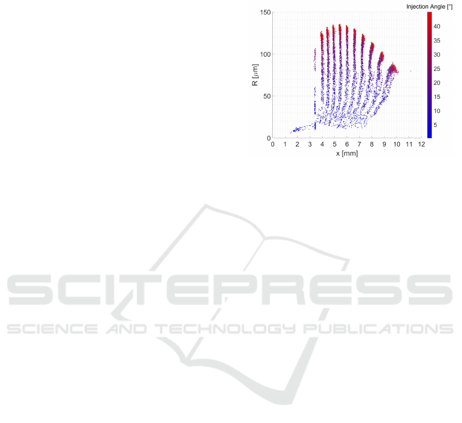
APPENDIX

Figure 13: Figure 10 with the particles colored by their In-

jection Angle θ.

Method for Automated Parametric Studies and Evaluation Using the Example of an Aerosol-on-Demand Jet-Printhead