Towards Computational Performance Engineering for

Unsupervised Concept Drift Detection:

Complexities, Benchmarking, Performance Analysis

Elias Werner

1,2 a

, Nishant Kumar

2,3 b

, Matthias Lieber

1,4 c

, Sunna Torge

1,2 d

Stefan Gumhold

1,2,3 e

and Wolfgang E. Nagel

1,2,4

Center for Interdisciplinary Digital Sciences (CIDS), Technische Universit

at Dresden, Germany

Center for Scalable Data Analytics and Artiﬁcial Intelligence (ScaDS.AI) Dresden/Leipzig, Germany

Chair of Computer Graphics and Visualization (CGV), Technische Universit

at Dresden, Germany

Center for Information Services and High Performance Computing (ZIH), Technische Universit

at Dresden, Germany

Keywords:

Concept Drift Detection, Performance Engineering, Complexities, Benchmark, Performance Analysis.

Abstract:

Concept drift detection is crucial for many AI systems to ensure the system’s reliability. These systems often

have to deal with large amounts of data or react in real-time. Thus, drift detectors must meet computational

requirements or constraints with a comprehensive performance evaluation. However, so far, the focus of de-

veloping drift detectors is on inference quality, e.g. accuracy, but not on computational performance, such

as runtime. Many of the previous works consider computational performance only as a secondary objective

and do not have a benchmark for such evaluation. Hence, we propose and explain performance engineering

for unsupervised concept drift detection that reﬂects on computational complexities, benchmarking, and per-

formance analysis. We provide the computational complexities of existing unsupervised drift detectors and

discuss why further computational performance investigations are required. Hence, we state and substantiate

the aspects of a benchmark for unsupervised drift detection reﬂecting on inference quality and computational

performance. Furthermore, we demonstrate performance analysis practices that have proven their effective-

ness in High-Performance Computing, by tracing two drift detectors and displaying their performance data.

1 INTRODUCTION

In the last years, the amount of available data in-

creased signiﬁcantly and is expected to be about

175 ZB only for the year 2025 (Reinsel et al., 2018).

The availability of vast amounts of data and the ex-

ploitation of computing resources such as graphics

processing units (GPUs) or tensor processing units

(TPUs) led to the emergence of deep learning (DL)

methods in many applications as predictive main-

tenance (Martinez et al., 2018), marine photogra-

phy (Langenk

amper et al., 2020), transportation plan-

ning (Grubitzsch et al., 2021) or computer vision

tasks such as object detection (Kumar et al., 2023).

https://orcid.org/0000-0003-2549-7626

https://orcid.org/0000-0001-6684-2890

https://orcid.org/0000-0003-3137-0648

https://orcid.org/0000-0001-9756-6390

https://orcid.org/0000-0003-2467-5734

However, many of these applications face differ-

ent challenges which concern 1.) the inference qual-

ity (e.g. accuracy) of the model and thus the effec-

tiveness of the application and 2.) the computational

performance of the application in terms of the com-

pute time and the compute resources.

The effectiveness of the applications is often de-

termined by the inference quality (e.g. accuracy) of

the DL model on a different data distribution than the

distribution which the model was trained with. How-

ever, while pure DL based applications work nicely

on the training data distribution, they might not per-

form as well when the test data distribution is differ-

ent from the training data distribution. Such changes

in the data distributions are referred to as concept

drift and are documented in many different applica-

tion ﬁelds. For example, (Grubitzsch et al., 2021)

outlined that the robustness of AI models is question-

able for sensor data-based transport mode recogni-

tion. The reason is the variety of context information,

318

Werner, E., Kumar, N., Lieber, M., Torge, S., Gumhold, S. and Nagel, W.

Towards Computational Performance Engineering for Unsupervised Concept Drift Detection: Complexities, Benchmarking, Performance Analysis.

DOI: 10.5220/0012758600003756

Paper published under CC license (CC BY-NC-ND 4.0)

In Proceedings of the 13th International Conference on Data Science, Technology and Applications (DATA 2024), pages 318-329

ISBN: 978-989-758-707-8; ISSN: 2184-285X

e.g. device type or user behavior that introduces con-

cept drift into the data. (Langenk

amper et al., 2020)

demonstrated concept drift when using different gear

or changing positions in marine photography and ex-

plained the effect on DL models. Hence, such appli-

cations need to be accompanied by approaches such

as concept drift detector (DD) to estimate changes in

the data distribution and to decide the robustness of

a DL model on a given input. DDs that require the

immediate availability of data labels are referred to

as supervised and DDs that reduce the amount of re-

quired data labels or can operate completely in the ab-

sence of labeled data are referred to as unsupervised.

The second challenge for applications is to han-

dle large amounts of data or high-speed data streams

and react in real-time. On the other hand, applica-

tions are often bound to certain hardware require-

ments or have to operate with limited computational

resources. These observations should point to the ne-

cessity of thorough investigations concerning com-

putational performance, i.e. runtime, memory usage,

and scalability. Thus, with DDs being an important

part of a robust DL pipeline, it is also necessary to

conduct such investigations on DDs. Note that we re-

fer to metrics as runtime or memory usage as compu-

tational performance and to metrics such as accuracy

or recall as inference quality. However, the literature

does not focus on computational performance inves-

tigations but concentrates on the methodological im-

provements and inference quality evaluation of DDs

on small-scale examples only as outlined in the survey

by (Gemaque et al., 2020). Moreover, while theoret-

ical computational complexities play a crucial role in

understanding algorithmic behaviors, they fall short

of encompassing the real-world performance of an al-

gorithm. This is attributed to various factors such as

implementation, compiler optimizations, data distri-

bution, and other external inﬂuences, which become

signiﬁcant when the algorithm operates on real hard-

ware and processes real data.

Our work focuses on unsupervised DDs that can

operate in the absence of data labels, as the provi-

sion of labeled training data is very expensive and

for many applications not given. So far, there

is no previous work comprehensively investigating

the computational performance of unsupervised DDs.

In response, our work reﬂects on the ﬁeld of per-

formance engineering, which has its roots in High-

Performance Computing (HPC) and introduces it for

unsupervised DDs. Thus, we discuss important pil-

lars for a comprehensive consideration of computa-

tional performance: complexity analysis, benchmark-

ing, and performance analysis. This work’s key con-

tributions include:

1. We reﬂect on the existing literature and show that

it lacks computational performance evaluation for

unsupervised concept drift detection.

2. We show a concrete path towards performance en-

gineering of DDs and discuss complexity analy-

sis, benchmarking, and performance analysis.

3. We provide the time and space complexities for a

set of existing DDs.

4. We state and substantiate the requirements for a

benchmark of unsupervised DD.

5. We demonstrate the effectiveness of performance

analysis tools by tracing two DDs and present the

performance data.

The rest of the paper consists of four parts. In Sec-

tion 2, we introduce preliminaries and deﬁne concept

drift. Section 3, provides an overview of the prior

works for unsupervised concept drift detection and

explains the scope of previous computational perfor-

mance evaluation. In Section 4, we introduce perfor-

mance engineering for unsupervised concept drift de-

tection. We provide computational complexities and

discuss them. Furthermore, we examine aspects for

a comprehensive benchmark and give initial insights

into performance analysis for DDs.

2 BACKGROUND

This section formally deﬁnes concept drift and intro-

duces supervised and unsupervised drift detection.

We follow the formal notations and deﬁnitions

by (Webb et al., 2016) for the following illustrative

equations, but also consider (Gama et al., 2014) and

(Hoens et al., 2012) among others. Note that our as-

sumptions hold for the discrete and continuous realms

in principle. Nevertheless, for ease of simpliﬁcation,

we consider only the discrete realm in our notations.

Assume for a machine learning (ML) problem there

is a random variable X over vectors of input features

, X

, ..., X

]. Moreover, there is a random variable

Y over the output that can be either discrete (for classi-

ﬁcation tasks) or continuous (for regression tasks). In

this case, P(X) and P(Y ) represent the probability dis-

tribution over X and Y respectively (priori). P(X , Y )

represents the joint probability distribution over X and

Y and refers to a concept. At a particular time t, a con-

cept can now be denoted as P

(X, Y ). Concept drift

refers to the change of an underlying probability dis-

tribution of a random variable over time. Formally:

(X, Y ) ̸= P

t+1

(X, Y ) (1)

Supervised drift detection is the process where the

Towards Computational Performance Engineering for Unsupervised Concept Drift Detection: Complexities, Benchmarking, Performance

Analysis

319

data labels Y are always immediately available and

unsupervised DDs detect drift without labeled data.

3 RELATED WORK

In the ﬁeld of supervised drift detection, different in-

vestigations by (Barros and Santos, 2018) and (Palli

et al., 2022) exist, that present and compare multiple

supervised DDs. Additionally, (Mahgoub et al., 2022)

presents a benchmark of supervised DDs that consid-

ers the runtime and memory usage of the related DDs

besides the DDs’ quality.

To the best of our knowledge, there is no

such benchmark for unsupervised DDs, Neverthe-

less, surveys exist that summarize the related work.

(Gemaque et al., 2020) and (Shen et al., 2023) pro-

vide overviews and taxonomies to classify unsuper-

vised drift detectors following different criteria. Al-

though both surveys mention the importance of com-

putational performance considerations, they did not

incorporate such objectives in their overviews thor-

oughly.

Investigating prior methods for unsupervised DDs

does also not provide enough evidence for thorough

computational performance investigations. Several

works (Mustafa et al., 2017; Kifer et al., 2004; Dit-

zler and Polikar, 2011; Haque et al., 2016; Sethi

and Kantardzic, 2017; Kim and Park, 2017; Zheng

et al., 2019; Cerqueira et al., 2022; Lughofer et al.,

2016; de Mello et al., 2019; G

uac¸ık et al., 2019;

uac¸ık and Can, 2021) do not conduct any runtime,

memory, energy or scalability performance measure-

ments. Thus, it is difﬁcult to assess their computa-

tional performance in real-world applications. Other

works by (Dasu et al., 2006; Gu et al., 2016; Lu

et al., 2014; Qahtan et al., 2015; Liu et al., 2017; Liu

et al., 2018; Song et al., 2007; dos Reis et al., 2016;

Greco and Cerquitelli, 2021; Pinag’e et al., 2020)

conduct few experiments concerning runtime on mul-

tiple datasets and compared their approaches to other

works sporadically. Only (Liu et al., 2018) investi-

gated memory utilization. In addition, not all papers

perform their evaluation with the same setting and

vary in the data sets chosen, the number and dimen-

sion of data points, and how the computational perfor-

mance measurements are carried out. Although some

works consider the theoretical computational com-

plexity of their algorithms, this can not replace empir-

ical measurements on real datasets and machines, e.g.

as shown by (Jin et al., 2012) highlighting the impact

of computational performance bugs on the runtime of

implementations. However, as discussed by (Lukats

and Stahl, 2023), source code is often not available

and the reproducibility of presented experiments is of-

ten questionable.

Future applications with high data volumes, high

data velocities, or computational resource constraints

will require resource-efﬁcient approaches and imple-

mentations. Contrarily, computational performance

aspects for unsupervised concept drift detection were

only investigated as a secondary objective in the liter-

ature. Thus, we require proper and well-documented

implementations that enable consistent computational

performance evaluations to assess the applicability

of DDs for use cases with high volumes and high-

velocity data. Moreover, to obtain resource-efﬁcient

AI systems and to avoid waste of resources, scalable

or parallel DDs and the resource-efﬁcient deployment

of the approaches need to be investigated. For such

developments, the HPC community has broad exper-

tise in the ﬁeld of performance engineering. Besides

computational complexity analysis and substantiated

best practices in benchmarking, several tools such as

Score-P (Kn

upfer et al., 2012) or Vampir (Kn

upfer

et al., 2008) are developed to support the system-

atic performance analysis of applications. Applying

these methods to unsupervised DDs supports the eval-

uation of the computational performance of differ-

ent approaches and allows systematically setting up

resource-efﬁcient solutions for future applications.

4 COMPUTATIONAL PERFOR-

MANCE ENGINEERING

In this section, we introduce our contributions to as-

sess the computational performance of unsupervised

DDs. This includes 1.) the computational complex-

ity of a set of DDs in Section 4.1, 2.) the concept

of a comprehensive benchmark in Section 4.2, and

3.) a clear workﬂow for performance analysis of DDs

in Section 4.3, exemplarily presented on two instru-

mented implementations.

As a motivating example, we randomly selected

the two unsupervised DDs Incremental Kolmogorov-

Smirnov (IKS) (dos Reis et al., 2016) and the student-

teacher approach STUDD (Cerqueira et al., 2022)

and measured the runtime and memory along with

the accuracy and amount of requested labels of

four pipelines: 1.) IKS: retraining of the base ML

model after drift detection with IKS 2.) STUDD: re-

training of the base ML model after drift detection

with STUDD 3.) Baseline 1 (BL1): pipeline with-

out re-training of the base ML model 4.) Baseline

2 (BL2): retraining of the base ML model after ev-

ery 5000 samples. IKS detects drift based on the

changes in the raw input data distribution by continu-

DATA 2024 - 13th International Conference on Data Science, Technology and Applications

320

100

IKS

STU DD

BL1

BL2

Accuracy (%)

100

IKS

STU DD

BL1

BL2

Labels (%)

5266

10218

4321

4432

12k

IKS

STU DD

BL1

BL2

Runtime(s)

704

1008

446

698

1.2k

IKS

STU DD

BL1

BL2

Memory(MB)

300

600

900

Figure 1: Accuracy, amount of labels, runtime, and peak

memory of the pipelines IKS, STUDD, BL1, and BL2 on

Forest Covertype dataset.

ously applying a Kolmogorov-Smirnov test on a ref-

erence dataset and a detection dataset. STUDD con-

sists of a student auxiliary ML model to mimic the

behavior of a primary teacher decision ML model.

Drift is detected if the mimicking loss of the student

model changes with respect to the teacher’s predic-

tions. All pipelines are implemented in Python and

use a Random Forest with 100 decision trees as the

base classiﬁer. The base classiﬁer is trained with the

ﬁrst 5000 samples of the dataset, the remaining data is

processed as a stream by the several pipelines. We ap-

plied all pipelines on the Forest Covertype (Blackard

and Dean, 1999) dataset that consists of 54 features

with seven different forest cover type designations in

5.8 ∗10

data samples. All experiments ran with a

single CPU core of an AMD EPYC 7702, ﬁxed to 2.0

GHz frequency. Note that since the implementations

do not run in parallel, we do not consider multiple

CPU cores. However, using HPC still offers advan-

tages for benchmarking over a local setup, such as a

ﬁxed CPU frequency and low system noise. In addi-

tion, we refer to best practices and methodologies in

the ﬁeld of HPC in this section. The source code of

the experiments for the depicted results will be avail-

able publicly

Our results are depicted in Figure 1. BL1 has the

lowest computational demand on the dataset, i.e. low-

https://github.com/elwer/Perf DD

est runtime and peak memory. However, it achieves

the lowest accuracy without requiring any further data

labels while processing the stream. BL2 has a slightly

higher computational demand than BL1 requests all

data labels due to the continuous re-training of the

base model and achieves much higher accuracy than

BL1. IKS consumes slightly more memory and run-

time than BL2. It achieves slightly higher accuracy

than BL2 while reducing the amount of required la-

bels by 50%. STUDD requires more memory than

the other pipelines and also the runtime is by far the

highest. It achieves a higher accuracy than BL1 but

lower than BL2. However, the strength of STUDD

is that the amount of requested labels is reduced to

only 3% of the total stream. Hence, we conclude that

for our setting, both DDs have their strengths: IKS

leads to a moderate reduction of requested labels by

preserving high accuracy without high computational

overhead. STUDD dramatically reduces the number

of requested labels by improving accuracy over BL1

at a high computational cost.

However, based on those measurements, it is un-

clear how DD based pipelines behave in different set-

tings since they highly rely on the chosen datasets, hy-

perparameters, or hardware constraints. (Barros and

Santos, 2018) demonstrated different behaviors of su-

pervised DDs on different datasets. Thus, we need

also a benchmark comprising different unsupervised

DDs. The Section 4.1. aims at an assessment of the

scaling behavior in space and time, and the complex-

ity results support the evaluation of the computational

performance of DDs in a benchmark.

4.1 Complexity Analysis

We determined the complexities for a set of DDs that

do not rely on a ML model or another method, that is

highly dependent on the underlying use case or data.

We determined the complexities based on the mathe-

matical foundations and pseudo-code presented in the

original works. Additionally, we aligned complexities

that have been presented in the literature according to

our notations. Finally, we state the complexities for

the approaches KL (Dasu et al., 2006), PR (Gu et al.,

2016), CD (Qahtan et al., 2015), NM-DDM (Mustafa

et al., 2017), HDDDM (Ditzler and Polikar, 2011),

IKS (dos Reis et al., 2016), BNDM (Xuan et al., 2020),

ECHO (Haque et al., 2016), OMV-PHT (Lughofer

et al., 2016), DbDDA (Kim and Park, 2017), CM (Lu

et al., 2014). See the Appendix for our justiﬁca-

tions of the outlined complexities. Although most ap-

proaches require an initialization phase for their drift

detection, the amount of data computed in this phase

is much smaller than the amount of data processing

Towards Computational Performance Engineering for Unsupervised Concept Drift Detection: Complexities, Benchmarking, Performance

Analysis

321

Table 1: Time and Space complexity per sample over

the data stream. Parameters: d: dimensions, w: win-

dow size, i.e examined data points, b: bins in histogram

(NM-DDM and OMV-PHT only), e: size of ensemble (Db-

DDA only), s: sampling times (NN-DVI only), δ: min-

imum value for the box length property (KL only).

Approaches: KL (Dasu et al., 2006), PR (Gu et al., 2016),

CD (Qahtan et al., 2015), NM-DDM (Mustafa et al., 2017),

HDDDM (Ditzler and Polikar, 2011), IKS (dos Reis et al.,

2016), BNDM (Xuan et al., 2020), ECHO (Haque et al.,

2016), OMV-PHT (Lughofer et al., 2016), DbDDA (Kim

and Park, 2017), CM (Lu et al., 2014).

Approach Time Complexity Space Complexity

KL O(d ×log(

)) O(w ×d)

PR O(log

w) O(w ×d)

CD O(d)

drift: O(d

×w)

O(w + d)

NM-DDM O(w ×d ×b) O(d ×b)

HDDDM O(⌊

√

w⌋×d) O(⌊

√

w⌋×d)

IKS O(log(w)) O(w ×d)

BNDM O(log(w)) O(w ×d)

ECHO O(w

) O(w)

OMV-PHT O(w + b) O(w + b)

DbDDA O(1)

ens.: O(e)

O(w)

ens.: O(e ×w)

CM O(w) O(w ×d)

the stream. Therefore, we skip the complexities of the

initialization phase and focus on the complexity per

sample while processing the stream.

Table 1 shows the time and space complexities of

the considered approaches when processing a stream.

Only ECHO has a quadratic time complexity with re-

spect to the window size, i.e. doubling w leads to qua-

drupling the runtime. CD has a quadratic time com-

plexity with respect to the dimensions of the data only

for the case of drift as reported in the original publi-

cation. Therefore, CD’s time complexity is dependent

on the nature of the data but also on the quality (ac-

curacy) of the drift detection itself, i.e. reporting too

much drift, leads to a high increase of the runtime.

KL is the only approach that depends only on the data

dimensions d and an internal parameter δ for main-

taining the data structure incrementally. The other

approaches’ time complexities depend on the window

size w directly, i.e. examined data points. The low-

est time complexity is determined for DbDDA by it-

eratively maintaining the mean and standard devia-

tion over the ML model conﬁdences in two windows

and comparing this to a threshold. Therefore, the time

complexity is constant, and for the ensemble case, the

number of ensemble members e. For the space com-

plexity, KL, PR, IKS, BNDM and CM store all the

data points, i.e. O(w ×d). ECHO and DbDDA rely

on w only since only one value per window needs to

be stored. For DbDDA ensemble, space complexity

grows proportionally with the ensemble size e and w.

Complexities are important pillars in analyzing a

DDs’ behavior concerning runtime and memory since

they highlight factors that inﬂuence time and space

complexity behaviors. However, they are not enough

to assess real-world scenarios on real data since the

complexities only reﬂect the scaling behavior but no

absolute runtimes or memory requirements. Thus,

even if the complexity of one approach is higher than

another one, better implementation and higher drift

detection accuracy might overcome this theoretical

drawback. Indeed, this should point to the necessity

of proper and optimized implementations, empirically

verifying the estimated theoretical complexities. Ad-

ditionally, the approaches’ detection accuracy is not

reﬂected in the time and space complexities at all.

Thus, we need empirical evidence reﬂecting on the

computational performance and quality as a crucial

additional investigation for concept drift detection.

4.2 Benchmarking

Conducting a benchmark in the ﬁeld of ML often

refers to comparing quality measures, e.g. accuracy or

recall of different approaches. Therefore, aiming for

computational performance as one main objective in

benchmarking faces particular challenges as initially

discussed in (Mattson et al., 2020). These particular

challenges are explained in this section with respect

to the ﬁeld of unsupervised concept drift detection.

Diversity in Datasets: The works identiﬁed in Sec-

tion 3 leverage different synthetic and real-world

datasets that are used to benchmark unsupervised

DDs. Synthetic data allows deﬁning drift patterns,

e.g. drift occurrence or frequency. Moreover, it is pos-

sible to deﬁne the kind of drift, i.e. virtual vs real

drift, or the temporal occurrence, e.g. abrupt, incre-

mental, gradual, or reoccurring (Webb et al., 2016).

For a benchmark, this has the advantage of having

a ground truth, we can compare drift detection re-

sults and create individual scenarios to reﬂect differ-

ent settings for drift detection. Examples of synthetic

data sources are Hyperplane (Hulten et al., 2001) or

Agrawal (Agrawal et al., 1993) among others, that are

implemented in the Massive Online Analysis (Bifet

et al., 2010) framework. However, the effectiveness

of using synthetic data depends on how well the data

represents real-world characteristics. This is empha-

DATA 2024 - 13th International Conference on Data Science, Technology and Applications

322

sized by (Souza et al., 2020) explaining the impor-

tance and challenges for benchmarking against real-

world data and providing a broad overview of avail-

able real-world datasets such as Abrupt Insects (dos

Reis et al., 2016), Gas (Vergara et al., 2012), Electric-

ity (Harries et al., 1999), Forest Covertype (Blackard

and Dean, 1999) or Airlines (Ikonomovska et al.,

2011). This is further afﬁrmed by (Gemaque et al.,

2020), referring to the fact that the amount of data

used for evaluating DDs is small across the whole lit-

erature. Furthermore, we recognized a big gap be-

tween the amount of data used for evaluating DDs

compared to benchmarks in the data streaming do-

main that use datasets with multiple million data

points, e.g. Amazon movie reviews (McAuley and

Leskovec, 2013) or Google web graph (Leskovec

et al., 2009). Additionally to data sizes, we propose

to reﬂect on class imbalances and multi-class data.

The multi-class scenario is given by many of the real-

world datasets, but should also be considered in syn-

thetic scenarios explicitly. (Palli et al., 2022) give ev-

idence on different behaviors of supervised DDs for

class imbalances in comparison to evenly distributed

class cases. They report similar results for multi-class

data in comparison to binary class. We need to extend

this research for unsupervised DDs.

Model Dependency: According to the survey

by (Shen et al., 2023), DDs can be separated into

two groups: A) differences in data distribution and

B) model quality monitoring. The latter can be con-

sidered model-dependent since it directly relies on a

model’s quality, whereas the ﬁrst group can be con-

sidered model-independent. For the model-dependent

approaches, we identify two cases of unreliable drift

detection. The ﬁrst case is when the model reports

high inference quality (e.g. high conﬁdence) after

concept drift, leading to wrong predictions but no

detection by the DD. Even if there are no studies

that prove this behavior in general, there are stud-

ies that prove it for selected models. E.g. (Nguyen

et al., 2015) provides evidence that deep learning

models produce high conﬁdence for incorrect predic-

tions, e.g. after concept drift. (Lughofer et al., 2016)

shows, that this is also the case for evolving fuzzy

classiﬁers. The second case is when the model reports

low inference quality (e.g. low conﬁdences) without

concept drift, leading to incorrectly detected drift and

unnecessary computational overhead due to subse-

quent drift handling strategies. Overﬁtting (Hawkins,

2004) could be a reason for such behavior, which ap-

plies to all types of ML models. Thus, we conclude,

due to the heterogeneity of ML models, it is impor-

tant to reﬂect on different base models for a bench-

mark comprehensively comparing DDs from groups

A and B.

Baselines: The literature often suggests no concept

drift detection as a baseline for a benchmark (Souza

et al., 2021; Cerqueira et al., 2022; dos Reis et al.,

2016). In particular, this refers to an initially trained

ML model that is not retrained during the process-

ing of a data stream, nor is any action beyond the

inference process considered. Therefore, this is the

best possible runtime for a given ML model and data

stream and does not require any further labeled data.

On the other hand, this baseline indicates the mini-

mum inference quality (e.g. accuracy) that a pipeline

with a DD should achieve. Thus, a second baseline

should reﬂect the best inference quality possible while

processing the stream by re-training the ML model af-

ter n samples. Therefore, it requires 100% of the true

labels. (Souza et al., 2021) deﬁnes n = 1 and retrains

the ML model after each sample. This results in a

very high runtime overhead for that pipeline due to

the permanent re-training of the ML model but guar-

antees the highest possible accuracy.

Additionally, we propose to consider at least one

more baseline. This is due to the asymptotic behav-

ior of the runtime and the differing behavior of the

inference quality, e.g. accuracy, while increasing n

that indicates the number of samples after which a

classiﬁer is re-trained while processing a stream. To

show this, we processed the ﬁve introduced datasets:

Abrupt Insects, Gas, Electricity, Forest Covertype and

Airlines. We implemented a Random Forest classiﬁer,

that is trained on initial data and updated every n sam-

ples. For the smaller datasets Abrupt Insects, Gas, and

Electricity we used 500 samples for the initial train-

ing, while for the bigger Forest Covertype and Air-

lines datasets, we used 2000 samples. We initialized

n = 1 and increased n by 5 for each run while pro-

cessing the small datasets. For the big ones, we ini-

tialized n = 20 and increased n by 100. Our results

are depicted in Figure 2. For all datasets, the run-

time strongly decreases while increasing n. Accuracy

decreases slowly for all datasets and higher n might

have a higher accuracy than lower n depending on the

dataset and how well the period of re-training matches

the drift pattern. In fact, we suggest a value of n

such that the runtime is low, while still maintaining

the high accuracy provided at the bend of the runtime

curve for all datasets.

(Cerqueira et al., 2022) deﬁnes n = 100, still

achieving high inference quality on their considered

datasets while heavily reducing the runtime overhead

since re-training is conducted only for each 100 sam-

ples. While this is a good starting point for a prag-

Towards Computational Performance Engineering for Unsupervised Concept Drift Detection: Complexities, Benchmarking, Performance

Analysis

323

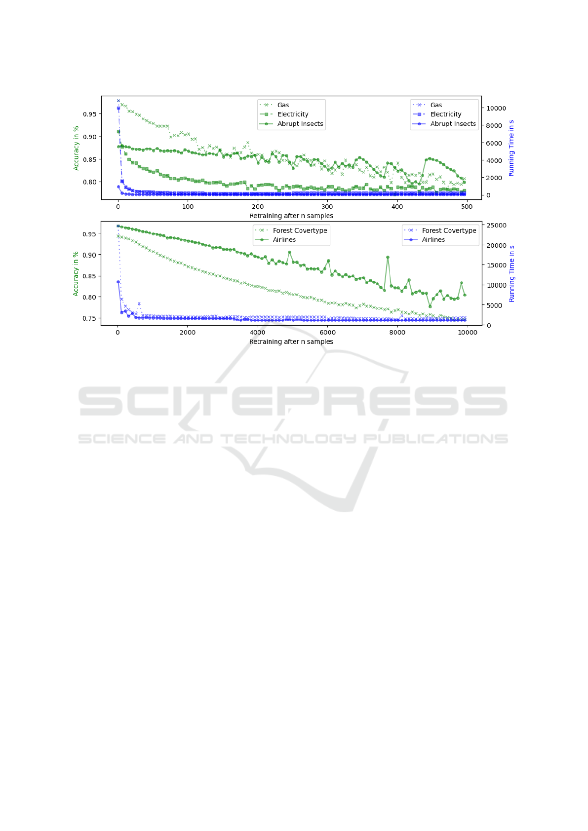
Figure 2: Accuracy and runtime behavior while processing streams over different datasets. The X-axis indicates the number of

samples after which re-training is conducted. The Y-axis (right/blue) shows runtime and Y-axis (left/green) shows accuracy.

Gas, Electricity, Abrupt Insects where initialized with n = 1 and sampled in steps of 5, Forest Covertype, Airlines were

initialized with n = 20 and sampled in steps of 100.

matic baseline, it might not be generally applicable

since it does not necessarily reﬂect on an optimum of

the curves, balancing accuracy and runtime. How-

ever, one can explore alternative values for n, i.e.

baselines depending on the dataset’s characteristics.

Set of Metrics: In (Barros and Santos, 2018), met-

rics to track the inference quality of a supervised

DD such as Accuracy, Precision, Recall, F1-Score,

True Positives, False Positives, Detection Delay, and

Mathew’s Correlation Coefﬁcient were used. Addi-

tionally, we propose to track the (cumulative) Accu-

racy Gain per Drift as presented by (Wu et al., 2021)

to measure the effectiveness of a DD throughout a

stream and not only once for the whole dataset. For

unsupervised DD we also suggest tracking the amount

of requested labels, since some DDs detect drift in

an unsupervised manner but request labels for subse-

quent actions. To track computational performance,

we propose metrics such as runtime, resource utiliza-

tion, and efﬁciency, i.e. memory or CPU utilization.

(Mahgoub et al., 2022) did a similar investigation and

tracked the runtime and memory of several supervised

DDs. As explained in (Mattson et al., 2020), in-

ference quality and computational performance can’t

be considered independently, since achieving higher

quality might also require further computational over-

head as we also showed in Figure 2. Thus, we pro-

pose two strategies: 1.) select a threshold or set a

target quality for the inference, and measure the com-

putational resources to achieve that 2.) set a thresh-

old for the runtime or memory and compute the infer-

ence quality (accuracy) that is achievable under this

resource constraints. As indicated by Table 1, a sim-

ilar runtime for two DDs might require different set-

tings for DD parameters, e.g. window size w.

We highlighted four main considerations required

for a comprehensive benchmark of unsupervised

DDs. However, one preliminary requirement is the

availability of proper implementations of the DDs, i.e.

without crucial performance bugs that deteriorate the

computational performance of the implementations as

outlined by (Jin et al., 2012). Nevertheless, as inves-

tigated by (Lukats and Stahl, 2023), implementations

are scarce, and prose details are often insufﬁcient for

proper re-implementations. This should point to the

necessity of the provision of proper descriptions or

implementations of the DDs by the community.

4.3 Performance Analysis

Performance analysis refers to testing, analyzing, and

optimizing systems to achieve computational perfor-

mance goals and to identify and resolve performance

DATA 2024 - 13th International Conference on Data Science, Technology and Applications

324

Figure 3: Vampir display of the IKS DD (left) and STUDD DD (right) performance data on the Forest Covertype dataset. In

each display, the left part shows the call tree and the right part shows the function summary, i.e. accumulated exclusive time

per function. User regions for the inference process are yellow, user regions for the drift detection are green, user regions for

maintaining buffers, and the ML model is red. sklearn functions are blue. The remaining functions are shaded grey.

bugs (Jin et al., 2012). It usually follows a two-step

workﬂow: 1.) proﬁling, i.e. accumulating perfor-

mance data, e.g. runtime of application functions or

memory 2.) tracing of an application to exactly record

program regions enter and exit over time. Both steps

support a performance analyst in identifying compu-

tational bottlenecks in implementations and improv-

ing an application’s behavior. For data science, it is

also crucial to reﬂect on the quality (e.g. accuracy)

when conducting performance analysis, emphasizing

the importance of holistic performance engineering,

e.g. improving the runtime behavior of an implemen-

tation while maintaining benchmark results. Score-

P (Kn

upfer et al., 2012) is an established, scalable

open-source framework that supports proﬁling and

tracing. With the Score-P Python bindings (Gocht

et al., 2021), it supports the Python programming

language, which can be considered predominant in

data science. Additionally, a Score-P Jupyter ker-

nel (Werner et al., 2021) makes it available for exe-

cution in Jupyter notebooks. Vampir (Kn

upfer et al.,

2008) is a tool to display performance data as col-

lected by Score-P.

To demonstrate the effectiveness of these work-

ﬂows, we measured the run of the two Python-

based DDs STUDD and IKS on the Forest Covertype

dataset. Figure 3 displays the performance data of

the STUDD and IKS run in Vampir. The left part

shows the call tree displaying the invocation hierar-

chy across the functions and accumulates the runtime.

The middle part displays a timeline of the called func-

tions (top) and their call stack (bottom). The right part

shows the function summary, i.e. accumulated exclu-

sive time per function. For both displays, we consider

user regions for the inference process (yellow), user

regions for the drift detection (green), user regions

for maintaining buffers, and the ML model (red). The

other functions are shaded grey.

For STUDD, we additionally colored sklearn

functions in blue and derived the following: As dis-

played in the function summary, the STUDD im-

plementation mostly relies on sklearn while pro-

cessing the stream. Based on the call tree, we see

that the time for drift detection (4780s, 76%) pre-

dominates over time for inference (1409s, 22%).

The call tree also shows the high dependency of

user:STUDD DriftDetetion on the sklearn base

functionalities. With these insights, we conclude that

the runtime overhead for STUDD is signiﬁcantly high

for processing the stream only due to the drift detec-

tion. This is mainly due to the approach of applying

and maintaining an additional student model. How-

ever, since it is mostly based on sklearn, which is

an established library with additional support for par-

allel execution, it is worth investigating how STUDD

scales across multiple cores or nodes.

For IKS, the most time for processing the pipeline

was spent on the inference process (1191s, 56%) as

shown in the call tree and the function summary. Nev-

ertheless, drift detection also takes 784s (37%) as

the call tree node user:IKS DriftDetetion shows.

This overhead is mostly based on the Add and Remove

functions of the IKS implementation, e.g. maintain-

ing the internal Treap data representation. The time

for maintaining the ML model and buffers can be

considered insigniﬁcant. With Vampir’s timeline

chart, it is possible to get further insights into chrono-

logical sequences of called functions. In Figure 4

we selected the period between the inference of two

subsequent samples of the data stream to investigate

IKS’ behavior per sample. We can see the recur-

sive call within IKS:Remove for removing the old-

est sample in the reference window. Subsequently,

the current sample is added and triggers a recur-

sive call within IKS:Add. Adding and removing a

sample mainly consists of a similar recursive se-

quence of methods, i.e. Treap:SplitKeepRight

(light green) at the beginning, Treap:Merge (dark

blue) at the end and either Treap:KeepGreatest

(cyan) or Treap:KeepSmallest (orange) in between.

Towards Computational Performance Engineering for Unsupervised Concept Drift Detection: Complexities, Benchmarking, Performance

Analysis

325

Figure 4: Vampir display of the IKS DD with timeline feature, i.e. chronological sequence of the called functions. We

selected the time window to show the called functions of the IKS per sample, i.e. between inference steps (yellow).

The top display shows the master timeline and the bottom display the call stack. Treap.SplitKeepRight is light green,

Treap.KeepGreatest cyan, Treap.KeepSmallest orange, Treap.Merge dark blue and other Treap functions are purple.

IKS:Add consists of additional merges.

Therefore, we conclude that IKS mostly relies

on the internal data representation. The resource-

efﬁcient and potentially parallel implementation of

maintaining this representation is the key to a low

runtime overhead. While we did not perform an in-

depth performance analysis of IKS and STUDD, we

still show the effectiveness of such investigations for

DDs. Further analysis should follow to support the

development of resource-efﬁcient scalable DDs.

5 CONCLUSION

This work contributes to computational performance

engineering for unsupervised DDs by discussing

computational complexities, a comprehensive bench-

mark, and an initial performance analysis of two DDs.

We show the necessity of such investigation by high-

lighting the gap in the prior evaluation and demon-

strating a high runtime of two DDs on a larger dataset.

Although time and space complexities alone are not

enough for comprehensive performance engineering,

they are an important pillar for such investigations.

Thus, we determined them for existing approaches.

The complexities can be reﬂected in a benchmark that

takes into account the important aspects we have dis-

cussed, i.e. diversity of datasets, model dependencies,

baselines, and the set of metrics. Performance anal-

ysis provides in-depth insights into application be-

haviors and supports the development of resource-

efﬁcient and parallel DDs. We provide an initial anal-

ysis with the tools Score-P and Vampir to reveal po-

tential bottlenecks in the implementations of two DD.

For future work, we plan to extend our com-

plexity analysis and substantiate the determined time

and space complexities with empirical measurements.

Moreover, we want to provide a comprehensive

benchmark of unsupervised DDs reﬂecting the com-

putational performance and inference quality. Us-

ing gained insights, we aim to develop parallel and

resource-efﬁcient solutions for diverse applications.

ACKNOWLEDGMENT

The authors gratefully acknowledge the computing

time made available to them on the high-performance

computer at the NHR Center of TU Dresden. This

center is jointly supported by the Federal Ministry

of Education and Research and the state governments

participating in the NHR (www.nhr-verein.de/unsere-

partner).

REFERENCES

Agrawal, R., Imielinski, T., and Swami, A. (1993).

Database mining: A performance perspective. IEEE

TKDE, 5(6):914–925.

Barros, R. S. M. and Santos, S. G. T. C. (2018). A large-

scale comparison of concept drift detectors. Informa-

tion Sciences, 451:348–370.

Bifet, A., Holmes, G., Pfahringer, B., Kranen, P., Kremer,

H., Jansen, T., and Seidl, T. (2010). Moa: Massive

online analysis, a framework for stream classiﬁcation

and clustering. In Proc. 1st Workshop on Applications

of Pattern Analysis, pages 44–50. PMLR.

Blackard, J. A. and Dean, D. J. (1999). Comparative ac-

curacies of artiﬁcial neural networks and discriminant

analysis in predicting forest cover types from carto-

graphic variables. Computers and Electronics in Agri-

culture, 24(3):131–151.

Cerqueira, V., Gomes, H., Bifet, A., and Torgo, L. (2022).

Studd: a student–teacher method for unsupervised

concept drift detection. Machine Learning, pages 1–

28.

Dasu, T., Krishnan, S., Venkatasubramanian, S., and Yi,

K. (2006). An information-theoretic approach to de-

tecting changes in multi-dimensional data streams. In

Proc. Symp. Interface.

de Mello, R. F., Vaz, Y., Grossi, C. H., and Bifet, A. (2019).

On learning guarantees to unsupervised concept drift

DATA 2024 - 13th International Conference on Data Science, Technology and Applications

326

detection on data streams. Expert Systems with Appli-

cations, 117:90–102.

Ditzler, G. and Polikar, R. (2011). Hellinger distance based

drift detection for nonstationary environments. In

IEEE Symp. CIDUE, pages 41–48. IEEE.

dos Reis, D. M., Flach, P., Matwin, S., and Batista, G.

(2016). Fast unsupervised online drift detection using

incremental kolmogorov-smirnov test. In Proc. 22nd

ACM SIGKDD Int. Conf. KDD, pages 1545–1554.

Gama, J.,

Zliobait

e, I., Bifet, A., Pechenizkiy, M., and

Bouchachia, A. (2014). A survey on concept drift

adaptation. ACM computing surveys, 46(4):1–37.

Gemaque, R. N., Costa, A. F. J., Giusti, R., and Santos,

E. M. D. (2020). An overview of unsupervised drift

detection methods. Wiley Interdisciplinary Reviews:

Data Mining and Knowledge Discovery, 10(6):e1381.

Gocht, A., Sch

one, R., and Frenzel, J. (2021). Advanced

python performance monitoring with score-p. In Tools

for High Performance Computing, pages 261–270.

Springer.

uac¸ık,

O., B

ukc¸akır, A., Bonab, H., and Can, F.

(2019). Unsupervised concept drift detection with a

discriminative classiﬁer. In Proc. 28th ACM Int. Conf.

CIKM, pages 2365–2368.

uac¸ık,

O. and Can, F. (2021). Concept learning us-

ing one-class classiﬁers for implicit drift detection in

evolving data streams. Artiﬁcial Intelligence Review,

54:3725–3747.

Greco, S. and Cerquitelli, T. (2021). Drift lens: Real-

time unsupervised concept drift detection by evaluat-

ing per-label embedding distributions. In Proc. IEEE

Int. Conf. ICDMW, pages 341–349. IEEE.

Grubitzsch, P., Werner, E., Matusek, D., Stojanov, V., and

ahnel, M. (2021). Ai-based transport mode recogni-

tion for transportation planning utilizing smartphone

sensor data from crowdsensing campaigns. In Proc.

IEEE 24th Int. Conf. ITSC, pages 1306–1313. IEEE.

Gu, F., Zhang, G., Lu, J., and Lin, C. (2016). Concept drift

detection based on equal density estimation. In Proc.

Int. Conf. IJCNN, pages 24–30. IEEE.

Haque, A., Khan, L., and M. Baron, B. Thuraisingham,

C. A. (2016). Efﬁcient handling of concept drift and

concept evolution over stream data. In Proc. IEEE

32nd Int. Conf. ICDE, pages 481–492. IEEE.

Harries, M., Wales, N. S., et al. (1999). Splice-2 compara-

tive evaluation: Electricity pricing.

Hawkins, D. M. (2004). The problem of overﬁtting. Jour-

nal of chemical information and computer sciences,

44(1):1–12.

Hoens, T. R., Polikar, R., and Chawla, N. V. (2012). Learn-

ing from streaming data with concept drift and imbal-

ance: an overview. Progress in Artiﬁcial Intelligence,

1:89–101.

Hulten, G., Spencer, L., and Domingos, P. (2001). Min-

ing time-changing data streams. In Proc. 7th ACM

SIGKDD Int. Conf. KDD, pages 97–106.

Ikonomovska, E., Gama, J., and D

zeroski, S. (2011). Learn-

ing model trees from evolving data streams. Data

Mining and Knowledge Discovery, 23:128–168.

Jin, G., Song, L., Shi, X., Scherpelz, J., and Lu, S. (2012).

Understanding and detecting real-world performance

bugs. ACM SIGPLAN Notices, 47(6):77–88.

Kifer, D., Ben-David, S., and Gehrke, J. (2004). Detecting

change in data streams. In Proc. 30th Int. Conf VLDB,

volume 4, pages 180–191. Toronto, Canada.

Kim, Y. and Park, C. H. (2017). An efﬁcient concept drift

detection method for streaming data under limited la-

beling. IEICE Transactions on Information and sys-

tems, 100(10):2537–2546.

upfer, A., Brunst, H., Doleschal, J., Jurenz, M., Lieber,

M., Mickler, H., M

uller, M. S., and Nagel, W. E.

(2008). The vampir performance analysis tool-set. In

Resch, M., Keller, R., Himmler, V., Krammer, B., and

Schulz, A., editors, Tools for High Performance Com-

puting, pages 139–155. Springer Berlin Heidelberg.

upfer, A., R

ossel, C., Mey, D., Biersdorff, S., Diethelm,

K., Eschweiler, D., Geimer, M., Gerndt, M., Lorenz,

D., Malony, A., et al. (2012). Score-p: A joint

performance measurement run-time infrastructure for

periscope, scalasca, tau, and vampir. In Proc. 5th Int.

Workshop on Parallel Tools for HPC, pages 79–91.

Springer.

Kumar, N.,

Segvi

c, S., Eslami, A., and Gumhold, S. (2023).

Normalizing ﬂow based feature synthesis for outlier-

aware object detection. In Proc. IEEE Conf. CVPR,

pages 5156–5165.

Langenk

amper, D., Kevelaer, R. V., Purser, A., and Nat-

tkemper, T. W. (2020). Gear-induced concept drift in

marine images and its effect on deep learning classiﬁ-

cation. Frontiers in Marine Science, 7:506.

Leskovec, J., Lang, K. J., Dasgupta, A., and Mahoney,

M. W. (2009). Community structure in large net-

works: Natural cluster sizes and the absence of large

well-deﬁned clusters. Internet Mathematics, 6(1):29–

123.

Liu, A., J.Lu, Liu, F., and Zhang, G. (2018). Accumulat-

ing regional density dissimilarity for concept drift de-

tection in data streams. Pattern Recognition, 76:256–

272.

Liu, A., Song, Y., Zhang, G., and Lu, J. (2017). Regional

concept drift detection and density synchronized drift

adaptation. In Proc. 26th Int. Conf. IJCAI.

Lu, N., Zhang, G., and Lu, J. (2014). Concept drift detec-

tion via competence models. Artiﬁcial Intelligence,

209:11–28.

Lughofer, E., Weigl, E., Heidl, W., Eitzinger, C., and

Radauer, T. (2016). Recognizing input space and tar-

get concept drifts in data streams with scarcely la-

beled and unlabelled instances. Information Sciences,

355:127–151.

Lukats, D. and Stahl, F. (2023). On reproducible implemen-

tations in unsupervised concept drift detection algo-

rithms research. In Proc. 43rd Int. Conf. SGAI, pages

204–209. Springer.

Mahgoub, M., Moharram, H., Elkafrawy, P., and Awad, A.

(2022). Benchmarking concept drift detectors for on-

line machine learning. In Proc. 11th Int. Conf. MEDI,

pages 43–57. Springer.

Towards Computational Performance Engineering for Unsupervised Concept Drift Detection: Complexities, Benchmarking, Performance

Analysis

327

Martinez, I., Viles, E., and Cabrejas, I. (2018). Labelling

drifts in a fault detection system for wind turbine

maintenance. In Proc. Conf. IDC XII, pages 145–156.

Springer.

Mattson, P., Cheng, C., Diamos, G., Coleman, C., Micike-

vicius, P., Patterson, D., Tang, H., Wei, G., Bailis, P.,

Bittorf, V., et al. (2020). Mlperf training benchmark.

volume 2, pages 336–349.

McAuley, J. J. and Leskovec, J. (2013). From amateurs to

connoisseurs: modeling the evolution of user exper-

tise through online reviews. In Proc. 22nd Int. Conf.

WWW, pages 897–908.

Mustafa, A. M., Ayoade, G., Al-Naami, K. W., Khan,

L., Hamlen, K., Thuraisingham, B., and Araujo, F.

(2017). Unsupervised deep embedding for novel class

detection over data stream. In Proc. IEEE Int. Conf.

Big Data, pages 1830–1839. IEEE.

Nguyen, A., Yosinski, J., and Clune, J. (2015). Deep neural

networks are easily fooled: High conﬁdence predic-

tions for unrecognizable images. In Proc. IEEE Conf.

CVPR, pages 427–436.

Palli, A. S., Jaafar, J., Gomes, H. M., Hashmani, M. A.,

and Gilal, A. R. (2022). An experimental analysis

of drift detection methods on multi-class imbalanced

data streams. Applied Sciences, 12(22):11688.

Pinag’e, F., dos Santos, E. M., and Gama, J. (2020). A drift

detection method based on dynamic classiﬁer selec-

tion. Data Mining and Knowledge Discovery, 34:50–

74.

Qahtan, A. A., Alharbi, B., Wang, S., and Zhang, X. (2015).

A pca-based change detection framework for multidi-

mensional data streams: Change detection in multidi-

mensional data streams. In Proc. 21st ACM SIGKDD

Int. Conf. KDD, pages 935–944.

Reinsel, D., Gantz, J., and Rydning, J. (2018). Data age

2025: the digitization of the world from edge to core.

Seagate.

Sethi, T. S. and Kantardzic, M. (2017). On the reliable de-

tection of concept drift from streaming unlabeled data.

Expert Systems with Applications, 82:77–99.

Shen, P., Ming, Y., Li, H., Gao, J., and Zhang, W. (2023).

Unsupervised concept drift detectors: A survey. In

Proc. 18th Int. Conf. ICNC-FSKD, pages 1117–1124.

Springer.

Song, X., Wu, M., Jermaine, C., and Ranka, S. (2007). Sta-

tistical change detection for multi-dimensional data.

In Proc. 13th ACM SIGKDD Int. Conf. KDD, pages

667–676.

Souza, V. M. A., dos Reis, D. M., Maletzke, A. G., and

Batista, G. E. (2020). Challenges in benchmarking

stream learning algorithms with real-world data. Data

Mining and Knowledge Discovery, 34:1805–1858.

Souza, V. M. A., Parmezan, A. R. S., Chowdhury, F. A.,

Mueen, A., and Abdullah (2021). Efﬁcient unsu-

pervised drift detector for fast and high-dimensional

data streams. Knowledge and Information Systems,

63:1497–1527.

Vergara, A., Shankar, V., Ayhan, T., Ryan, M. A., Homer,

M. L., and Huerta, R. (2012). Chemical gas sensor

drift compensation using classiﬁer ensembles. Sen-

sors and Actuators B: Chemical, 166-167:320–329.

Webb, G., Hyde, R., Cao, H., Nguyen, H., and Petitjean,

F. (2016). Characterizing concept drift. Data Mining

and Knowledge Discovery, 30(4):964–994.

Werner, E., Manjunath, L., Frenzel, J., and Torge, S. (2021).

Bridging between data science and performance anal-

ysis: tracing of jupyter notebooks. In Proc. 1st Int.

Conf. AIMLSys, pages 1–7.

Wu, O., Koh, Y. S., Dobbie, G., and Lacombe, T. (2021).

Nacre: Proactive recurrent concept drift detection in

data streams. In Proc. Int. Conf. IJCNN, pages 1–8.

IEEE.

Xuan, J., Lu, J., and Zhang, G. (2020). Bayesian nonpara-

metric unsupervised concept drift detection for data

stream mining. ACM TIST, 12(1):1–22.

Zheng, S., Zon, S., Pechenizkiy, M., Campos, C., Ipenburg,

W., and Harder, H. (2019). Labelless concept drift

detection and explanation. In Proc. Workshop Robust

AI in FS.

APPENDIX

We justify the determined time and space complexi-

ties. All approaches refer to at least two parameters:

w - window size (number of examined data points)

and d - number of data dimensions per data point.

KL (Dasu et al., 2006) δ - minimum value for the

property box length of their internal data representa-

tion kdq-tree State the time and space complexity

in the publication.

PR (Gu et al., 2016) State the time complexity

of their approach in the publication. For the space

complexity, they store w instances with d features, i.e.

O(w ∗d)

CD (Qahtan et al., 2015) Even not mentioned ex-

plicitly in their publication, processing a sample relies

on the data dimensionality d since the projection of a

data point onto the PCs is done in O(d ×k), where

k is the number of PCs describing 99.9% of the vari-

ance and k can be considered as a constant. For drift,

they report O(d

×w). Space complexity for the PCs

with a ﬁxed k is O(d) and O(w) due to the projection

of the data points in the reference window on a ﬁxed

number of PCs, i.e. O(w + d).

NM-DDM (Mustafa et al., 2017) b - number of

bins of estimated histogram State the time com-

plexity of their approach in the publication. For the

space complexity, b number of bin values in each of

the histograms for the d features are stored, i.e. d ∗b.

HDDDM (Ditzler and Polikar, 2011) Originally

HDDDM was proposed as a batch-based approach.

To apply it incrementally on each sample, we as-

sume a naive procedure: we introduce an initialization

DATA 2024 - 13th International Conference on Data Science, Technology and Applications

328

phase over the ﬁrst samples S

with i = 1, 2, ...w and

initialize D

= D

= S

, ...S

. For each new sample

and t = w +1, w +2, ..., we initialize D

= D

t−1

∪S

t−w

to create a sliding window of size w. Now, we

apply the HDDDM as usual.

Drift detection is performed by Hellinger dis-

tances between two histograms based on S

and S

The histograms have ⌊

√

w⌋ bins and the main com-

putational complexity is in the Hellinger distance be-

tween these two histograms, i.e. O(⌊

√

w⌋× d) to

compute the intermediate distances per bin of each

feature, resulting in the ﬁnal Hellinger distance. For

space complexity, only the histograms must be kept

in memory, i.e. O(⌊

√

w⌋×d).

IKS (dos Reis et al., 2016) State the time com-

plexity of their approach in the publication. For the

space complexity, they store w instances with d fea-

tures, i.e. O(w ∗d)

BNDM (Xuan et al., 2020) State the time com-

plexity of their approach in the publication. For the

space complexity, they store w instances with d fea-

tures, i.e. O(w ∗d)

ECHO (Haque et al., 2016) State the time and

space complexity of their approach in the publication.

OMV-PHT (Lughofer et al., 2016) b - number

of bins of estimated histogram Propose an exten-

sion of the Page-Hinkley test by only considering de-

teriorations of the quality indicator (e.g. accuracy)

and fading older samples for computing the quality

indicator. Besides a supervised quality indicator, they

propose a semi-supervised one, that relies on active

user feedback, and an unsupervised quality indica-

tor which is considered in this study. To determine

the quality of a model, they build histograms over the

model conﬁdence values during inference. Next, they

compare the histograms of two windows by iterating

over the bins, i.e. O(b), and apply their faded Page-

Hinkley test in O(w) since the fading of older samples

needs to be re-computed. An update of the histograms

can be done per sample in O(1). Therefore, the over-

all time complexity is O(w + b). Space complexity is

O(w + b) to store the conﬁdence histogram and the w

magnitude values for the OMV-PHT test.

DbDDA (Kim and Park, 2017) Calculates mean

and standard deviation for a reference and detection

window of size w over the conﬁdences of the ML

model in the inference. Mean and standard deviation

are computed iteratively in O(1) per dimension with

space complexity O(w) to store all conﬁdences. The

reference window is either ﬁxed or moving for Db-

DDA. For the ensemble case, multiple reference win-

dows are kept, and mean and standard deviation are

considered w.r.t. this ensemble, i.e. time complexity

O(e) and space complexity O(e ∗w).

CM (Lu et al., 2014) State the time complexity

of their approach in the publication. For the space

complexity, they store w instances with d features, i.e.

O(w ∗d).

Towards Computational Performance Engineering for Unsupervised Concept Drift Detection: Complexities, Benchmarking, Performance

Analysis

329