Inﬂuential Factors on Drivetrain Consumption in Electric City Buses and

Assessing the Optimization Potentials

Sunilkumar Raghuraman

1,2 a

, Daniel Baumann

2 b

, Marc Schindewolf

2 c

and Eric Sax

2 d

Daimler Busses, Mannheim, Germany

Karlsruhe Institute of Technology, Karlsruhe, Germany

Keywords:

Electric City Bus, Drivetrain Energy Consumption, Inﬂuencing Factors, Drive Style Analysis, Clustering.

Abstract:

In response to the growing need for sustainable mobility amidst global challenges like climate change and

urbanization, ensuring energy-efﬁcient operation of Electric City Buses (ECBs) is crucial. This study initially

utilizes techniques associated with explainable artiﬁcial intelligence, such as SHapley Additive ExPlanations

(SHAP), to determine the impact of various factors such as vehicle speed, acceleration, braking on drive-

train consumption. The data is categorized into distinct scenarios such as acceleration, starting, curve, uphill

and downhill for this analysis. In driving scenarios such as curves, uphill, or downhill, the position of the

brake pedal, along with the accelerator pedal and vehicle speed, were identiﬁed as signiﬁcant factors affecting

drivetrain consumption. Secondly, the study delves into analyzing driving behavior during bus stop entries,

employing methods like Deep Autoencoder-based Clustering (DAC) and Self-Organizing Map (SOM). In the

results of the DAC and SOM analysis, it was found that Cluster 2, identiﬁed through the DAC model, ex-

hibited substantial energy consumption, characterized by higher acceleration and lesser brake pedal usage.

Conversely, the SOM analysis showed that the orange and blue clusters have greater energy efﬁciency, with

a higher distance covered and lower energy consumption, contrasting with other clusters that consumed more

energy for reaching the busstop.

1 INTRODUCTION

Given the challenges posed by global warming, pop-

ulation growth, and urbanization, the automotive

industry faces mounting demands to foster more

sustainable mobility. Electrifying vehicles offer a

promising solution to mitigate greenhouse gas emis-

sions in transportation. An increasing shift can also be

observed in public transportation, where diesel-fueled

buses are being replaced by electric city buses (ECB)

(Mahmoud et al., 2016). ECBs now account for up to

4% of all new bus registrations in Europe, where elec-

tric bus registrations have been rising steadily since

2016 (IEA, 2021). In 2021, for the ﬁrst time, three

European countries registered more than 500 e-buses,

with Germany leading the way with 581 units, fol-

lowed by the UK with 540 units and France with 512

(SustainableBus, 2023). By 2022, nearly 66,000 elec-

https://orcid.org/0009-0001-5929-9567

https://orcid.org/0009-0004-4270-3713

https://orcid.org/0000-0002-2638-4861

https://orcid.org/0000-0003-2567-2340

tric buses and 60,000 medium and heavy-duty trucks

will have been sold worldwide, representing about

4.5% of all bus sales and 1.2% of truck sales world-

wide (IEA, 2023). At the same time, the transport

companies already have concrete plans to produce

around 6,600 more e-buses by 2030.

The energy consumption of an ECB consists of

many components, namely drivetrain, heating, venti-

lation and air conditioning (HVAC), 24V Auxiliary,

and Air compressor. The top two consumers are the

drivetrain and HVAC (R

osch et al., 2023). An es-

sential aspect of energy consumption estimation is

considering the impact of driver’s range anxiety, par-

ticularly the avoidance of driving with minimal en-

ergy remaining in the battery. It is important to note

that the actual energy consumption of electric buses

varies considerably depending on factors which are

not directly controllable or alterable, such as pas-

senger load, weather and trafﬁc conditions However,

driving style, which can be adjusted and optimized,

offers an avenue to improve energy efﬁciency in elec-

tric buses. Utilizing the real world ﬂeet data helps

in identifying possibilities for energy efﬁcient oper-

330

Raghuraman, S., Baumann, D., Schindewolf, M. and Sax, E.

Inﬂuential Factors on Drivetrain Consumption in Electric City Buses and Assessing the Optimization Potentials.

DOI: 10.5220/0012758700003756

Paper published under CC license (CC BY-NC-ND 4.0)

In Proceedings of the 13th International Conference on Data Science, Technology and Applications (DATA 2024), pages 330-337

ISBN: 978-989-758-707-8; ISSN: 2184-285X

ation for the top consumers such as drivetrain and

HVAC (Sommer et al., 2023).

This research paper aims to investigate the various

factors that impact drivetrain consumption in electric

city buses and explore the opportunities for optimiz-

ing energy efﬁciency. By analyzing real-world data,

and considering relevant parameters, this work aim to

provide valuable insights into the key determinants of

drivetrain consumption in ECBs. Furthermore, this

study will assess how different driving styles, partic-

ularly scenarios like bus stop approaches, inﬂuence

drivetrain efﬁciency. By examining these interactions,

we aim to identify strategies for optimizing drivetrain

performance in electric city buses.

2 BACKGROUND

2.1 Explainable Artiﬁcial Intelligence

Explainable Artiﬁcial Intelligence (XAI) aims to en-

hance the transparency of AI systems, moving away

from opaque ”black box” models towards algorithms

that provide interpretable insights into decision-

making processes. XAI seeks to make AI systems

clearer and more trustworthy by offering explicit ex-

planations that outline their capabilities, limitations,

and behaviors in unfamiliar situations.The SHAP

method (SHapley Additive ExPlanations), rooted in

cooperative game theory and speciﬁcally Shapley val-

ues, measures the impact of each input feature on

a model’s prediction. It calculates Shapley values

by considering all possible combinations of features,

assessing their effect on the prediction. These val-

ues highlight the importance of each feature, with

positive values indicating beneﬁcial contributions and

negative ones showing negative effects (Lundberg and

Lee, 2017).

2.2 Deep Autoencoder-Based Clustering

Deep Autoencoder-based Clustering (DAC) (Lu and

Li, 2021) is a generalized data-driven framework to

learn to cluster representations using deep neuron net-

works. The methodology described in the study by Lu

et al. involve training a deep autoencoder, consisting

of an encoder and a decoder, using a provided training

set. They initiated the process with a ﬂattened input

vector fed into a three-layer deep encoder, which is

crucial for obtaining a low-dimensional learned repre-

sentation. This representation was then reconstructed

to its original dimensions by the decoder. Once their

auto-encoder was adequately trained, it was used to

produce a low-dimensional representation of the input

data, which was then employed as input for the K-

Means clustering algorithm to establish the required

clusters in the data.

2.3 Self-Organizing Map

Kohonen’s SOM (Kohonen, 1990) algorithm was em-

ployed in this study to model the dataset. It is an ar-

tiﬁcial neural network algorithm that operates on the

principles of competitive learning. In SOM, an initial

grid of neurons is established, each initialized with

random vectors matching the input data’s dimensions.

During training, input data points are presented ran-

domly to these neurons, with each neuron competing

to become the Best Match Unit (BMU) by calculat-

ing its distance to the input. The BMU and its neigh-

boring neurons adjust their codebook vectors based

on a learning function. This process is repeated over

the entire training set, resulting in centroids dispersed

throughout the data space. After training, the nodes

can be visualized in a grid structure, that helps in un-

derstanding the relationships and patterns.

3 RELATED WORK

Although ECB are environmental-friendly and able to

beneﬁt the development of a sustainable urban tran-

sit system, an important concern is energy consump-

tion estimation that relates to driver’s range anxi-

ety—avoid driving with little energy remaining in the

battery. In recent years, numerous researches have

focused on developing more energy-efﬁcient driving

styles (Zhang et al., 2019; Kivek

as et al., 2019; He

et al., 2021) and assistance systems to enhance the

performance of an ECB. In a simulation study, a two-

part strategy was developed in determining an optimal

velocity interval (30-40 km/h) and an energy-saving

acceleration mode, which resulted in a reduction of

energy consumption by 2.47% overall in a bus trip

in the simulation (Zhang et al., 2019). On the other

hand, in this study efﬁcient design choices were sug-

gested to reduce the energy consumption (Kivek

et al., 2019).

ECB’s energy consumption is inﬂuenced by sev-

eral factors, including road geometry, land use,

weather, and vehicle conditions, as well as the driving

behavior. Although vehicle conditions, weather, land

use, and road geometry are typically constant factors

within a predeﬁned bus route, the driving style can

vary among different drivers.

Predicting the energy consumption or determin-

ing the inﬂuencing factors are divided into two types,

named as macroscopic and microscopic approaches

Inﬂuential Factors on Drivetrain Consumption in Electric City Buses and Assessing the Optimization Potentials

331

(Chen et al., 2021). The macroscopic approach fo-

cuses on developing models that predict energy con-

sumption for longer distances of operation (Varga

et al., 2019; Zhang et al., 2020; Thorgeirsson et al.,

2021). It aims to estimate the overall energy con-

sumption of an electric vehicle for the whole trip of

operation. Additionally, this approach is utilized to

predict the remaining range that will be covered by

the vehicle, providing valuable information for plan-

ning and optimization. These studies have utilized

inﬂuential factors, related to vehicle design, driver-

related parameters, and environmental conditions as

well.

The microscopic approach primarily focuses on

the prediction of instantaneous energy consumption,

which deals with second by second basis of the con-

sumption (Zhang and Yao, 2015; De Cauwer et al.,

2017; Beckers et al., 2020). This methodology also

incorporates a wide array of factors, including driv-

ing conditions, vehicle speed, acceleration, and the

activation of auxiliary systems. By taking these vari-

ables into consideration, the microscopic approach

offers insights into the energy consumption patterns

and dynamics exhibited by electric vehicles during

their real-time operation.

4 METHODOLOGY

The methodology adopted in this study is structured

into two distinct phases. The initial phase focuses on

identifying the factors that signiﬁcantly impact driv-

etrain consumption, speciﬁcally in certain scenarios.

Subsequently, the second phase analyzes the driving

behavior and consumption patterns as buses approach

and enter the bus stops.

To determine the main inﬂuencing factors for the

power consumption in the bus, a 1D-Convolutional

Neural Network model (cf. (Kiranyaz et al., 2021))

was trained to predict the energy consumption for the

next time step from various input signals. The trained

model was then analyzed using SHAP to extract the

various inﬂuencing factors on the drivetrain energy

consumption (cf.Figure 1).

Figure 1: Workﬂow of getting the inﬂuencing factors of the

drivetrain.

Table 1: Criteria for the seven scenarios to identify the in-

ﬂuencing factors of the drivetrain.

Scenario

Group

Acceleration

x-Direction

Acceleration

y-Direction

Height Difference

Brake Pedal

Accelerator Pedal

Vehicle Speed

[m/s

] [m/s

] [m] [%] [%] [km/h]

Acc 1 > 0.2 > 0.01 < 15

Starting 1 > 0 < 5 > 0.01 < 15

Curve 2 > 0.7 > 5

Uphill 2 > 0.01 > 0.00

Downhill 2 < −0.01 > 0.01

The pipeline, we used to prepare the data and train

the model, is based on the CRISP-DM process (Wirth

and Hipp, 2000). The data used for the training and

prediction are measurement data collected utilizing

onboard data collectors installed in electric city buses.

In the data preparation stage, the dataset was parti-

tioned into separate subsets for subsequent analysis,

and individual trips within the time series data were

identiﬁed by utilizing GPS coordinates of the depot

location. This identiﬁcation was crucial for isolating

discrete journey segments, subsequently leading to a

comprehensive feature selection process. The rele-

vant features were selected, removing highly corre-

lated signals and signals irrelevant to get the inﬂuenc-

ing factors of the drivetrain. We trained a model with

the following input features to predict the drivetrain

energy consumption:

• Brake torque

• Ignition state

• Total distance

• Speed

• Brake pedal

• Accelerator pedal

• Vehicle weight

• Remaining range

• Cruise control

• Current gear

• Air temperature inside

• Air temperature outside

• Steering wheel

• Battery voltage

• Retarder level

• Current energy consumption

• Battery isolation resistance

• Road level

• Inverter 1/2 power

• Low voltage output power

• Acceleration in x/y

• left/right turn signal

• Actual high voltage power

• Brake system malfunction

• Stop request

• Horn

The last 5 seconds were used as the time window for

the input signals. The label value for the model is

the current power value of the drivetrain consump-

tion. Considering the whole dataset, 70% of the data

is used as training, 20% is used for validation, and

10% is used for testing the model. Before training the

model, the different windows of the training data were

balanced.In doing so, the naturally underrepresented

(very high and very low values cf. Figure 2 orange)

energy consumption is oversampled; for this purpose,

DATA 2024 - 13th International Conference on Data Science, Technology and Applications

332

the underrepresented data samples are repeated in the

data (cf. Figure 2 blue). Thereby an equal distribution

of the training windows across all energy consump-

tion is achieved (cf. Figure 2).

Figure 2: Histogram of the Train (before and after oversam-

pling), Test and Validation Data.

For the explanation of the evaluation step, the data

has been categorized into ﬁve scenarios to determine

the inﬂuencing factors and to avoid comparing dis-

similar situations (cf. Table 1). In this study, we have

organized the scenarios into two groups to facilitate a

clearer presentation of results (cf. Table 1). The sce-

narios of the ﬁrst group differ essentially in the initial

speed of the vehicles. Whereby the scenarios of the

second group only differ in their form of driving.

For each of the ﬁve scenarios, heatmaps based on

GPS coordinates were generated to identify locations

with frequent occurrences. The ﬁve locations with the

highest concentration of data points were further in-

vestigated. Data from these locations were processed

and aggregated into separate datasets for each sce-

nario. These datasets were then analyzed using SHAP

values to identify key inﬂuencing factors.

In the second phase of the driving behavior anal-

ysis, focused on bus stop entry. Initially, timestamps

for entering bus stops are determined after a trip re-

duction phase using speciﬁc signals such as GPS co-

ordinates, vehicle speed, and door status. These sig-

nals serve as key criteria for identifying instances

where the vehicle halts at a bus stop. Instances where

the vehicle speed reaches zero and the door status

opens at the GPS locations are isolated for further ex-

amination.

Subsequently, an extensive set of features is ex-

tracted for analysis purposes, which are categorized

into two types, as detailed in Table 2. They form a

vector of twenty seconds capturing time-based com-

ponents indicating different aspects of driving behav-

ior. This results in a high-dimensional feature rep-

resentation that offers a comprehensive insight into

driving behavior during bus stop entry. Using these

feature vectors, two distinct clustering techniques,

DAC and SOM, are employed.

Table 2: Features used for clustering + identifying bus

stops.

Method Feature Unit Type

Identifying bus stop

Door status

Latitude degrees

Longitude degrees

Clustering

Velocity m/s Vector of 20

Acc. Pedal % Vector of 20

Brake Pedal % Vector of 20

Drivetrain Energy kWh Scalar

Distance Traveled km Scalar

In this study, we employed the Supersom method-

ology to organize input variables into layers with as-

signed weights. Data on velocity, acceleration, and

brake pedal usage were segmented into vectors rep-

resenting twenty-second intervals, while distance and

energy per kilometer were treated as scalars in a sepa-

rate layer. The trained Supersom created a map where

each maneuver was represented by a hexagon. These

hexagons were then used as inputs for the K-means

clustering algorithm to determine clustering results,

assessing the optimal cluster number by analyzing

the elbow point in the within-cluster sum of squares

(within

) from 2 to 20 clusters. The ”kohonen” pack-

age was utilized to visualize the SOM model, present-

ing one layer of the codebook vectors at a time.

5 RESULTS AND DISCUSSION

5.1 Inﬂuential Factors of the Drivetrain

Energy Consumption

Our research aims to comprehensively understand and

analyze the factors that inﬂuence drivetrain energy

consumption. To achieve this, we employ SHAP val-

ues as a powerful tool for feature attribution.

As Group 1 only differ in the initial speed of the

vehicle, the inﬂuencing factors of the two scenarios

only differ slightly. The two main factors inﬂuencing

the drive energy are the acceleration pedal and vehi-

cle speed (cf. Figure 3). The Figure shows the mean

values of the absolute Shap values for a GPS position

in the starting scenario for the respective inﬂuencing

factors.The energy requirement increases with higher

speeds and higher acceleration. Therefore, it is nec-

essary to allocate more power resources to sustain ac-

celeration and maintain the desired velocity.

As Group 2 describes situations in which the ve-

hicle is driving, the most inﬂuencing factors for the

drivetrain energy are similar to Group 1, the acceler-

Inﬂuential Factors on Drivetrain Consumption in Electric City Buses and Assessing the Optimization Potentials

333

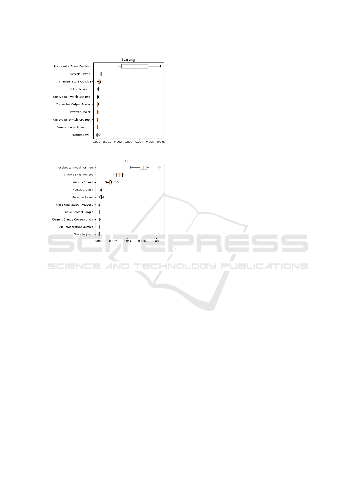
Figure 3: Top ten factors in the starting scenario.

Figure 4: Top ten factors in the Uphill scenario.

ator and brake pedal position as well as the vehicle

speed. These parameters can be explained physically,

e.g. the increased driving resistance at higher speeds

(cf. Figure 4). Firstly, the position of the accelerator

pedal remains a critical determinant. The degree to

which the accelerator is pressed directly impacts the

amount of energy delivered to the drivetrain, inﬂuenc-

ing the vehicle’s speed and acceleration.

Secondly, the brake pedal position plays a cru-

cial role in the energy dynamics of the drivetrain.

When the brake pedal is engaged, it signiﬁes a reduc-

tion in the vehicle’s speed. Conversely, releasing the

brake pedal allows for the restart of the energy ﬂow,

facilitating acceleration. Thirdly, the vehicle speed

emerges as another pivotal factor within this scenario

group. The speed at which the vehicle is traveling

is integrally linked to both the accelerator and brake

pedal actions. Higher speeds generally require more

energy to maintain. Besides the brake pedal, another

signiﬁcant factor inﬂuencing drivetrain energy con-

sumption is the retarder, that is installed in the electri-

cal vehicle. In addition to the primary braking mech-

anism provided by the brake pedal, the retarder level

serves as an additional braking.

In addition to the top 10 parameters shown in Fig-

ure 3 and Figure 4, there are other parameters, that

inﬂuence the drivetrain energy. The battery voltage

also plays a role, since higher battery voltage results

in lower energy consumption due to reduced losses

from the lower currents required to meet the same

power demands when compared to lower voltage sit-

uations.

The remaining range also affects the drivetrain en-

ergy, as position seven in the acceleration scenario

and position 15 in the starting scenario. This may be

due to the fact that drivers tend to be more aware of

energy consumption when the remaining range is low.

In these situations, individuals are likely to pay closer

attention to their driving habits, adjusting their behav-

ior to optimize energy efﬁciency as they strive to max-

imize the remaining distance they can cover with the

available energy.

5.2 Bus Stop Based Cluster Analysis

The dataset spans January to December 2022 and in-

cludes around 45,000 instances of electric city buses

arriving at stops, sourced from ten buses across cities

with varying altitudes. The Analysis reveals an aver-

age speed of 20.89 km/h with a standard deviation of

9.02 km/h, showing signiﬁcant speed variance. Ad-

ditionally, the mean positions of the acceleration and

brake pedals in the last twenty seconds reaching the

bus stop were found to be 18.69% (4.07-54.92%) and

14.03% (1.57-44.21%), respectively; notably, the ac-

celeration value of 54.92% appears to be an outlier.

Instances with more than 10 seconds of missing en-

ergy consumption data at any bus stop were excluded,

focusing the study on driving style and its impact on

energy consumption

5.2.1 Results of DAC

In the application of the DAC model, along with K-

means clustering, the data was segmented into three

distinct clusters, labeled as Cluster IDs 0, 1, and 2

(cf.Figure 5). In this clustering, Cluster 2 came as

the group with substantial energy consumption (Bad

Cluster), as evidenced by its higher drivetrain en-

ergy metrics per kilometer (Comparison with Cluster

0: 2.024 kWh/km higher, Cluster 1: 1.481 Kwh/km

higher). Conversely, Cluster 0 is recognized as a

cluster with reduced energy consumption, exhibit-

ing the least energy per kilometer with a negative

value among the clusters indicating more recuperation

(Good Cluster) (Comparison with Cluster 2: 2.024

kWh/km lower, Cluster 1: 0.543 Kwh/km lower).

Cluster 1 displays intermediate energy consumption,

higher than Cluster 0 but lower than Cluster 2 (Com-

parison with Cluster 0: 0.543 kWh/km higher, Cluster

DATA 2024 - 13th International Conference on Data Science, Technology and Applications

334

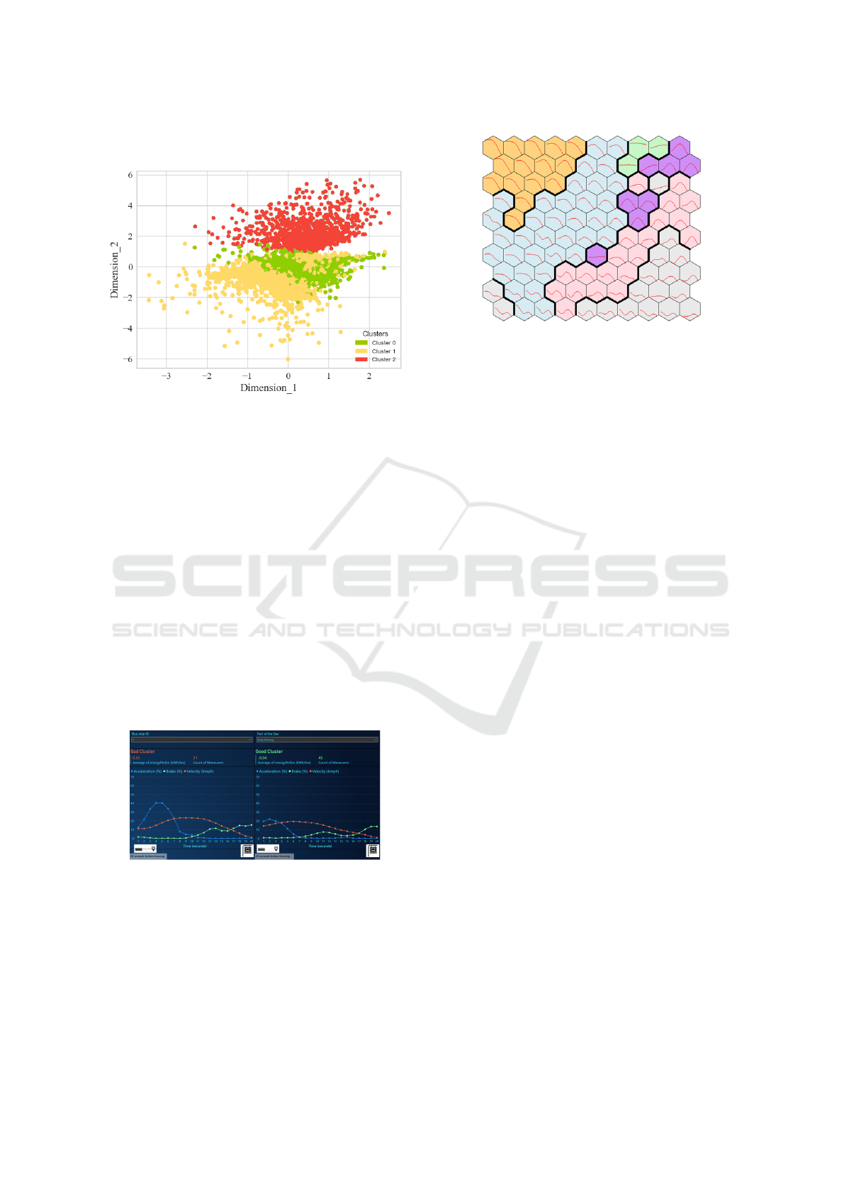
2: 1.481 Kwh/km lower).

Figure 5: Three clusters resulted from the DAC and Kmeans

clustering.

The high consumption cluster (Cluster 2), reveals

a pattern of lesser brake pedal usage coupled with

elevated acceleration values. This combination con-

tributes to increased energy consumption and dimin-

ished energy recuperation. Vehicles in this cluster

were noted to maintain lower speeds in previous time

instances, necessitating increased acceleration to ar-

rive at bus stops in a timely manner. This pattern is

observable not only during times of heavy trafﬁc but

also during early morning and late-night hours in the

same bus stop in different time instances, as depicted

in cf.Figure 6 and indicated as the bad cluster (Cluster

2). Given that these periods typically witness reduced

trafﬁc, the driving pattern may be more reﬂective of

individual driver behaviors or ignorance of the driver

to follow energy efﬁcient driving than external trafﬁc

conditions.

Figure 6: Driving style at early morning time period on dif-

ferent days at a speciﬁc bus stop.

Conversely, Cluster 0, which is characterized by

the lowest energy consumption per kilometer, shows

a different pattern in terms of brake and accelera-

tion. The average brake pedal usage in this cluster

is 69.75% higher than that in Cluster 2. Moreover,

the acceleration observed in Cluster 0 is consistently

lower compared to that in the high-consumption clus-

Figure 7: Code map for the vector layer Speed (kmph).

ter. Ultimately, the contrast between the clusters of-

fers insights into the diverse strategies drivers employ

and their impact on energy usage.

5.2.2 Results of SOM

The SOM analysis was conducted using a 10x10

hexagonal grid, resulting in a total of 100 hexagons.

Each hexagon in the code map corresponds to a

unique node in the SOM, depicting distinct driving

behaviors observed in the data. To determine the op-

timal clustering of these behaviors, an elbow curve

analysis was utilized, which identiﬁed six as the ideal

number of clusters. Therefore, the hexagons in the

code map have been color-coded into six different cat-

egories, each representing a cluster. Equal weighting

was assigned to all three vector layers and the singular

scalar layer during the training phase of the SOM.

Upon analyzing the velocity map in cf. Figure 7,

it was observed that in the orange and blue clusters,

there was a gradual decrease in speed over the twenty-

second time frame. In contrast, the pink and purple

clusters exhibited a distinct pattern where the speed

initially increased from a low point, peaked, and then

decreased again, forming a trajectory similar to a half-

circle as described in cf. Figure 7. The grey clus-

ter was characterized by generally lower speed values

and exhibited little variation. In the ﬁnal green cluster,

a consistently high speed was maintained throughout

the observed period.

In the acceleration map analysis, distinct patterns

emerged across the clusters (cf. Figure 8). The

orange, blue, and green clusters predominantly dis-

played a decreasing trend in acceleration values, re-

maining largely within a lower range. A notable ex-

ception was identiﬁed within the blue cluster, where

a peak in acceleration was observed in approximately

ﬁve hexagons. In stark contrast, the pink and pur-

ple clusters exhibited a pronounced sudden peak in

acceleration, which later subsided. This pattern sug-

gests a more dynamic and variable acceleration be-

Inﬂuential Factors on Drivetrain Consumption in Electric City Buses and Assessing the Optimization Potentials

335

havior in these clusters. The grey cluster, however,

presented a more nuanced pattern of acceleration, os-

cillating from low to high and then reverting to low,

yet these ﬂuctuations were conﬁned to a lower range

and did not exhibit the high peaks seen in the pink and

purple clusters.

Figure 8: Code map for the vector layer Acceleration (%).

In the orange and blue clusters of the brake pedal

code map (cf. Figure 9), braking was applied con-

sistently in the last twenty seconds before a bus stop,

with brake values decreasing over about twelve sec-

onds. In contrast, the pink and purple clusters showed

predominant braking in the last ﬁve seconds, effective

due to generally lower speeds. The grey cluster exhib-

ited a more irregular braking pattern; in eight speciﬁc

hexagons, two distinct peaks in brake value were ob-

served, indicating variable braking behavior. Mean-

while, the green cluster showed a consistent brake

value of zero, suggesting no change or application of

the brakes in this cluster. These patterns highlight di-

verse braking strategies inﬂuenced by speed and ap-

proach to bus stops.

Figure 9: Code map for the vector layer Brake pedal (%).

Analyzing the scalar component code map in cf.

Figure 10, which details distance and energy use

over twenty seconds, clear energy efﬁciency pat-

terns emerged. The orange and blue clusters demon-

strated greater efﬁciency, consuming 0.697 and 0.606

kWh/km less than the highest consumption cluster, re-

spectively, achieving more distance (≈ 270 m) with

less energy. In contrast, the purple, pink, gray, and

green clusters consumed more energy (0.528, 0.426,

0.457, and 0.697 kWh/km higher, respectively) for

shorter distances (≈ 120 m), indicating lower energy

efﬁciency.

Figure 10: Code map for the scalar layer, depicting the dis-

tance traveled and energy consumed.

A count plot analysis (cf. Figure 11) of these

clusters indicated a higher frequency of instances in

hexagons that were less energy efﬁcient, suggesting

that certain driving styles lead to increased energy

consumption during bus stop approaches. Alterna-

tively, this pattern may also reﬂect a lack of aware-

ness or concern among drivers regarding more efﬁ-

cient driving methods. The orange and blue clusters

are characterized by a negative average energy value

which is negative, indicative of effective energy recu-

peration as the bus approaches the stop. Within the

dataset, 20,875 instances, constituting 45.86% of the

total observed bus stop entries, fall into the energy-

efﬁcient clusters. Meanwhile, the clusters identiﬁed

as less energy efﬁcient comprise 24,642 instances,

which equate to 54.14% of the entire set of data

points.

6 CONCLUSION

In summary, this research utilizes SHAP values to

comprehensively analyze drivetrain energy consump-

tion. Two distinct scenario groups were identiﬁed:

one focuses on acceleration and starting, while the

other focuses on various driving conditions. Ac-

celeration is primarily inﬂuenced by the accelerator

pedal and vehicle speed, with higher speeds demand-

ing more energy. In driving scenarios, factors such as

accelerator and brake pedal positions, vehicle speed,

and retarder level play crucial roles.

DATA 2024 - 13th International Conference on Data Science, Technology and Applications

336

Figure 11: Number of driving instances entering the bus

stop mapped into different nodes.

The DAC analysis disclosed that the cluster with

elevated drivetrain energy consumption exhibited in-

creased acceleration upon approaching bus stops, a

trend which is also prevalent during early morning

and nighttime periods. Likewise, the SOM analysis

determined that more than half of the instances in the

dataset fell into clusters characterized by energy in-

efﬁciency, thereby contributing to sub-optimal energy

consumption.

By adjusting driving behaviors and reducing in-

efﬁcient practices, the operational efﬁciency of city

buses can be signiﬁcantly improved. Future research

could explore the nuances of energy consumption as

electric city buses transition from idling to motion,

particularly when departing from bus stops. This

analysis would complement current ﬁndings and pave

the way for the development of data-driven systems

to help drivers optimize energy use during operations.

REFERENCES

Beckers, C. J., Paroha, M., Besselink, I. J., and Nijmeijer,

H. (2020). A microscopic energy consumption pre-

diction tool for fully electric delivery vans. (5).

Chen, Y., Wu, G., Sun, R., Dubey, A., Laszka, A., and

Pugliese, P. (2021). A review and outlook of energy

consumption estimation models for electric vehicles.

De Cauwer, C., Verbeke, W., Coosemans, T., Faid, S., and

Van Mierlo, J. (2017). A data-driven method for

energy consumption prediction and energy-efﬁcient

routing of electric vehicles in real-world conditions.

Energies, 10(5).

He, Y., Li, J., Chen, Z., Wu, C., Ba, J., and Li, Z. (2021).

Research on identiﬁcation approach of risky driving

behaviors for new energy vehicles based on internet

of vehicles data. In 2021 6th International Confer-

ence on Transportation Information and Safety (IC-

TIS), pages 1320–1326.

IEA (2021). Global ev outlook 2021: Scaling up the transi-

tion to electric mobility.

IEA (2023). Trucks and buses - international energy agency.

Accessed on 2023.12.08.

Kiranyaz, S., Avci, O., Abdeljaber, O., Ince, T., Gabbouj,

M., and Inman, D. J. (2021). 1d convolutional neu-

ral networks and applications: A survey. Mechanical

Systems and Signal Processing, 151:107398.

Kivek

as, K., Lajunen, A., Baldi, F., Veps

ainen, J., and

Tammi, K. (2019). Reducing the energy consumption

of electric buses with design choices and predictive

driving. IEEE Transactions on Vehicular Technology,

68(12):11409–11419.

Kohonen, T. (1990). The self-organizing map. Proceedings

of the IEEE, 78(9):1464–1480.

Lu, S. and Li, R. (2021). Dac: Deep autoencoder-based

clustering, a general deep learning framework of rep-

resentation learning.

Lundberg, S. and Lee, S.-I. (2017). A uniﬁed approach to

interpreting model predictions.

Mahmoud, M., Garnett, R., Ferguson, M., and Kanaroglou,

P. (2016). Electric buses: A review of alternative pow-

ertrains. Renewable and Sustainable Energy Reviews,

62(C):673–684.

osch, T., Raghuraman, S., Sommer, M., Junk, C., Bau-

mann, D., and Sax, E. (2023). Multi-layer approach

for energy consumption optimization in electric buses.

In 2023 IEEE 97th Vehicular Technology Conference

(VTC2023-Spring), pages 1–6.

Sommer, M., R

osch, T., and Sax, E. (2023). Fleet data

used for self-learning functions in commercial vehi-

cles. In 17th International Conference Commercial

Vehicles 2023, page 81.

SustainableBus (2023). Electric bus public transport: Main

ﬂeets and projects around the world. Accessed on

2023-12-08.

Thorgeirsson, A. T., Scheubner, S., F

unfgeld, S., and Gau-

terin, F. (2021). Probabilistic prediction of energy

demand and driving range for electric vehicles with

federated learning. IEEE Open Journal of Vehicular

Technology, 2:151–161.

Varga, B. O., Sagoian, A., and Mariasiu, F. (2019). Pre-

diction of electric vehicle range: A comprehensive re-

view of current issues and challenges. Energies, 12(5).

Wirth, R. and Hipp, J. (2000). Crisp-dm: Towards a stan-

dard process model for data mining. In Proceedings of

the 4th international conference on the practical ap-

plications of knowledge discovery and data mining,

volume 1, pages 29–39. Manchester.

Zhang, J., Wang, Z., Liu, P., and Zhang, Z. (2020). Energy

consumption analysis and prediction of electric vehi-

cles based on real-world driving data. Applied Energy,

275:115408.

Zhang, R. and Yao, E. (2015). Electric vehicles’ energy

consumption estimation with real driving condition

data. Transportation Research Part D: Transport and

Environment, 41:177–187.

Zhang, Y., Yuan, W., Fu, R., and Wang, C. (2019). Design

of an energy-saving driving strategy for electric buses.

IEEE Access, 7:157693–157706.

Inﬂuential Factors on Drivetrain Consumption in Electric City Buses and Assessing the Optimization Potentials

337