Reputation, Sentiment, Time Series and Prediction

Peter Mitic

Department of Computer Science, UCL, London, U.K.

Keywords:

Reputation, Sentiment, Time Series, Prediction, Auto-Correlation, ARIMA, Cholesky, C opula, Normal

Mixture Distribution, Goodness-of-Fit, TNA Test.

Abstract:

A formal formulation for reputation is presented as a time series of daily sentiment assessments. Projections of

reputation time series are made using three methods that replicate the dist r ibutional and auto-correlation prop-

erties of the data: ARIMA, a Copula ﬁt, and C holesky decomposition. Each projection is tested for goodness-

of-ﬁt with respect t o observed data using a bespoke auto-correlation test. Numerical results show that Cholesky

decomposition provides optimal goodness-of-ﬁt success, but overestimates the projection volatility. Express-

ing reputation as a time series and deriving predictions fr om them has signiﬁcant advantages in corporate ri sk

control and decision making.

1 INTRODUCTION

The title gives the ﬂavour of this study in the order

of its words. Reputatio n is derived from Sentime nt

as a Time Series which is used for Prediction. The

sequence starts with wanting to know about product

and company perfo rmance.

There has been a huge increase since ye ar 2000

in interest in and progress with the analysis of peo-

ples views on products and services, fuelled by tech-

nological advances (Liu, 2015). Increased develop-

ment of th e internet, the rise of on-lin e media (both

social and ’traditio nal’ - newspapers and b roadcast-

ing), has made it possible for consumers to formulate

their own views on products and services in advance

of m a king a decision on purchase or use. Fundamen-

tal to such decision making is the concept of reputa-

tion. Informally, reputation is ”the opinion that peo-

ple in gene ral have about someone or something, or

how much respect or admiration someone or so me-

thing receives, based on past behaviour or character”

(Cambridge, 2023). The same reference gives an in-

formal deﬁnition for sentiment: ”a thought, opinion,

or idea based on a feeling about a situation, or a way

of thinking about something”. We will give f ormal

deﬁnitions fo r both in Section 3.4. The informal deﬁ-

nitions are, however, remarkably close to the ideas we

wish to convey formally. We will distinguish between

reputation, sentiment and opinion, and link them in a

formal way.

https://orcid.org/0000-0002-9845-4435

The purpose of this paper is to p redict how the

reputation of a corporate body may develop in the

future. Reputation is expressed as a time series, to

which time ser ie s methods apply naturally. However,

reputation tim e series express distinct characteristics

which makes it difﬁcult to apply standard m ethods

without some degree of conditioning. In particular,

they are highly auto-c orrelated, are sub je ct to rapid

reversals in proﬁle (they look ’spiky’), exhibit hig h

volatility, and are not always stationary. Others have

sparse, or almost no sentim ent expression. Reputation

time series are built using expressions of sentiment,

so an initial discussion sets out formal deﬁnitions f or

sentiment and reputation.

We consider predicted reputation because there is

some evidence that ”reputation means money” (Cole,

2012), (Weber-Shandwick, 2020). On that basis,

reputation was quantiﬁed in terms of share price in

(Mitic, 2024). Speciﬁcally, impaired reputation can

lead to effects such as loss of proﬁt, share price re-

duction, and reduced ability to attract and retain staff.

These, and similar reports are not quantiﬁed in a

transparent way, but nevertheless convey the message

that a positive reputation matters. Consequen tly, pre-

dicting future reputation also matters.

1.1 Reputation Time Series Example

In this section we show an example of a re putation

time series. Figure 1 shows Toyota’s reputation for

the ﬁrst 6 months of 2023, and a simple exponential

Mitic, P.

Reputation, Sentiment, Time Series and Prediction.

DOI: 10.5220/0012762600003756

Paper published under CC license (CC BY-NC-ND 4.0)

In Proceedings of the 13th International Conference on Data Science, Technology and Applications (DATA 2024), pages 51-61

ISBN: 978-989-758-707-8; ISSN: 2184-285X

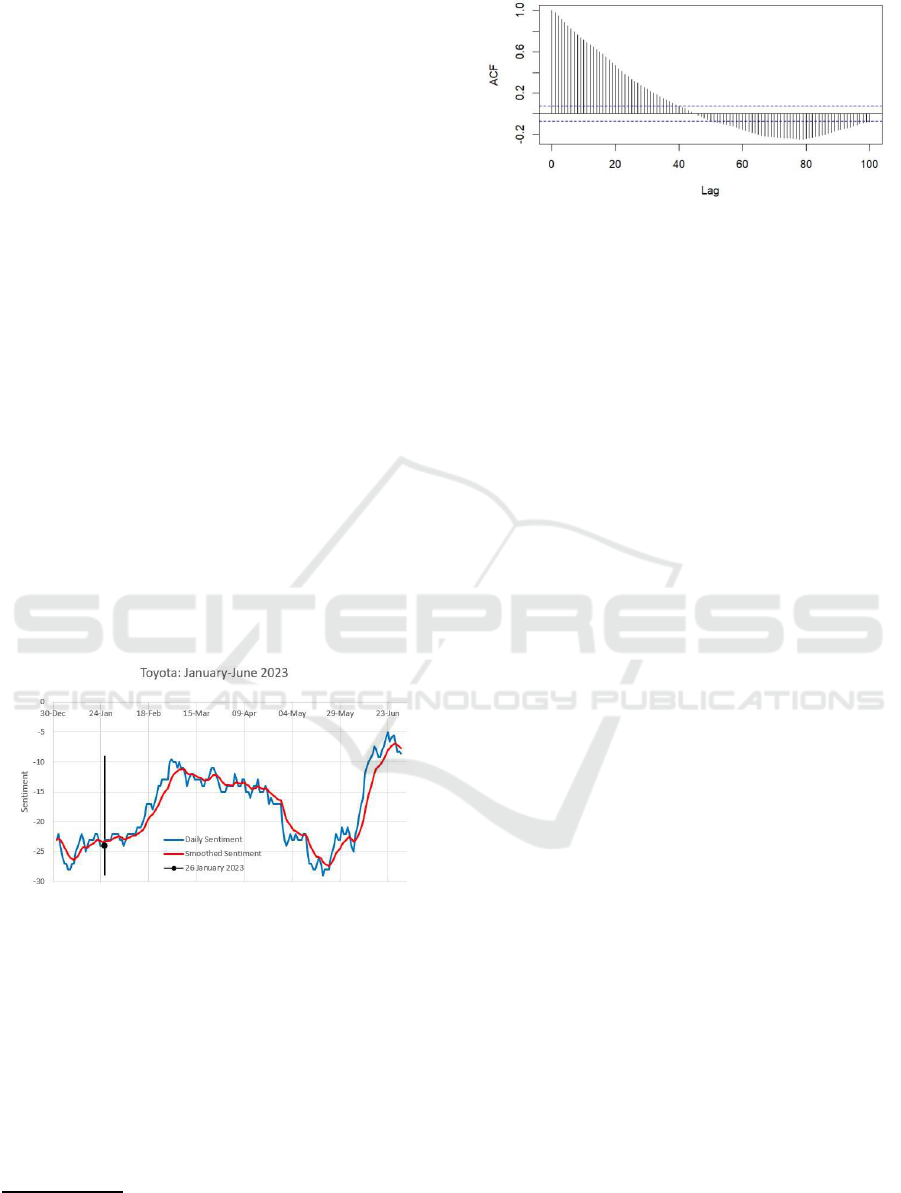
smoothed version of it. The plot shows time, m e a-

sured in days, on the horizontal axis, and numerical

expressions of sentiment on the vertical axis on a

scale -100 to +100. The tra ce shows that during that

period, Toyota’s reputation was entirely negative.

To see why, would require detailed analysis o f each

sentiment value, but a major contributor was the

change of Toyota’s leadership. That news was widely

reported in th e ﬁnancial press at the time. A typical

example, which is part of a longer article, a ppeared

in a Reuters repor t on 26 January 2023.

Reactions to Akio Toyoda stepping down as Toyota

CEO. TOKYO, Jan 26 (Reuters) - Toyota Motor

Corp (7203 .T) said on Thursd ay that Ak io Toyoda

will step down as president and chief executive to

become chairm a n fr om April 1, ...

Figure 1 shows the date 26th January 2023. Inter-

estingly, reputation improved after that date, perhaps

indicating that the news was received positively, al-

though that rise did not last long. The reputation trace

shows typical features: peaks and troughs in a macro-

structure, with a micro-structure of muc h smaller vari-

ations. Toyota’s autocorre la tion struc ture is shown in

Figure 2. The plot shows typical features of signiﬁ-

cant au tocorrelatio ns at high lags, with some positive

and negative regions.

Figure 1: Toyota reputation January-June 2023. Data

source: Penta Group.

2 RELATED WORK

Reputation time series as described in Section 3.4

are a natu ral extension of much earlier work on

opinion, sourced by survey. The ﬁrst pro minent

example of a survey was a correct prediction of

the 1936 US Presidential election by the Gallup

Company (founded in 1935) (Gallup an d Rae,

https://www.reut ers.com/business/autos-transportatio

n/toyota-leader-akio-toyoda-s tep-down-president-chi ef-e

xecutive-2023-01-26/

Figure 2: Toyota autocorrelation: 100 lags.

1968), although there is a record of an op inion

poll from 1824 in the Harrisburg Pennsylvanian

(https://www.referenceforbusiness.com/history2/

84/The- G allup-Organization.html). G a llup took the

view that a n opinion poll was simply a reﬂection

of public opin ion. There is an interesting counter

opinion due to Lippman (Lippman, 1922) that

opinion polls manipulate public opinion. The point

is discussed in (Jacobs and Shapiro, 1995). In 1995

the internet was relatively young, but since then

the means to manip ulate opinion have emerged in

the fo rm of blogs, social media platforms (such as

Facebook, WhatsApp or Twitter (”X”)), and produc t

reviews on websites such as Amazon, Google and

others. Problems of sample bias are discussed in

(Durant, 1954). They centre on location, respondents,

and questionnaire design, with additional factors

related to administration, cost, and whether or not the

results represent a g eneral population.

There is evidence of bias in c ontemporary opin-

ion procurement. The term ’negative bias’ was intro-

duced by (Rozin and Royzman, 2001), and clear nu-

merical illustrations are presented in (Zendesk, 2013).

Early research on sentiment and opinion is sum-

marised in, for example, (Das and Chen, 2007). The

emphasis was then on sentiment extraction using lex-

icons (word lists with tags showing related words

or parts of speech), lexical grammar (rules for ma-

nipulating a lexicon), and classiﬁers (Bayes, Voting,

Naive, Vector-Distance, Discrimin ant). Those meth-

ods still for m the basis of ’traditional’ sentiment anal-

ysis, and act as a benchmark for assessing later ap-

proach e s using artiﬁcial in telligence.

Prediction of reputation has, to date, been some-

what neglected, largely because of a lack of appro-

priate d ata. The problem was tac kled, albeit in a dif-

ference sense of the word ’prediction’ by (Loke and

Kachaniuk, 2020), using a bi-dir ectional LSTM. That

study u sed manual labelling of thousands of product

reviews, evaluated on a 3-point scale, aimed at pre-

dicting individual review results. Our study aims to

produce a forward proje ction in time, and uses much

simpler prediction methods. Penta Group, as part

DATA 2024 - 13th International Conference on Data Science, Technology and Applications

of their reputation intelligence web site

available to

subscribers, shows a basic forward (in time) predic-

tion based on exponential smoothing.

2.1 Alternative Sources of Reputation

Intelligence

In this section we summarise the state of online Repu-

tation Intelligence. The term Reputation Intelligence

has been used in the past ten years to refe r more gen-

eral aspe cts of sentiment and reputation. A reputa-

tion time series is one of them. Others include, for

example, analysis of sentiment sources (e.g. tradi-

tional/social media), analysis of r egional sentiment,

compariso n with peers, a nd Environmental, Social

and Governance (ESG) issues.

Artiwise, produced by Istanbul Technical Uni-

versity (https://www.artiwise.com) provides (to sub-

scribers) bespoke sentiment analysis services, and

calculates a short-term sentiment score based on

a limited number of sources to order. The Cali-

fornian company Reputation (https://reputation.com/)

provides the same type of service, and makes a

Reputatio n Experience Management - RXM platform

available to customers. In New York, Social360

(https://www.social360monitoring.com) p rovides be-

spoke a nalysis of online comments, and tracks inﬂu-

ential reporting ag e nts. Th ey specialise in social me-

dia checking. Social360 has recently be acquired by

(SignalAI, 202 4).

An earlier, and different, approach is typiﬁed by

the RepTrak Pulse metric (Fombrun et al., 2015),

published twic e yearly by th e Reputation Institute

(https://www.reptrak.com/). Rep Trak is an updated

version of its predecessor, the Reputa tion Quo-

tient (Fomb run et al., 2000) . Both are multi-

factor snapshot assessments of reputa tion. Rep-

Trak Pulse exports ”Good overall reputation”, ”Good

feeling about”, ”Trust”, and ”Admire and Respect”,

all condensed comments amassed throughout the

six months prior to publication. In contrast, the

Net Promoter S core - NPS from Bain and Co.

(https://www.bain.com/) is very simple, but limited

(Reichheld, 2003). It is b ased on one question: On

a scale of 0-10, how likely are you to recommend this

compan y to a friend or colleague?. The NPS is th en

the difference between the percentage of 9-10 (pro-

moter) scores and the percentage of 0-6 scores (de-

tractors). Score s 7 and 8 are r egarded as ”passive”.

The imbalance appears to induce negative bias. The

study by ( Loke and Reitter, 2 021) used the same ty pe

of multi-factor analysis to measur ing reputation, us-

https://pentagroup.co/

ing online review data and ’aspect’ extraction by de-

tecting negative sentiment and positive sentiment key-

words.

A third strand of r e putation measurement is

demonstra te d by the Edelman Trust Barometer

(https://www.edelman.com). Trust is so mewhat dis-

tinct fro m sentiment or reputation, and implies a de-

gree of safe ty and/or reliability (Cambridge, 2023).

The Edelman method of data sourcing is, again, by

survey, targeted at employees, and produce s gener-

alised qualitative reports, with some a ssoc iate d data.

An examp le is (Russell, 2023). The argument in

(Renner, 2011) is that risk can be minimised by in-

creasing trust, and that corp orate r eputation is the ve-

hicle to build trust.

A few other attempts to measure reputation have

emerged. (Janson, 2014) r ecommends spending at

least 1 0% of a corporate budget on reputation al anal-

ysis and sampling, but is oth erwise non-speciﬁc on

methodology. (Carreras et al., 2013) suggests a rank-

ing method in which c ompany executives rank them-

selves and peers o n a multi-factor basis, and produce a

score based o n those ranks. Overall, these and similar

alternatives rely on the subjective opinion of selected

individuals.

3 METHODS

We ﬁrst review data stationarity and a methodo logy

for measuring the appropriate ness of a projected time

series. Three projection methods are then discu ssed :

ARIMA, Copula and Cholesky.

3.1 Stationarity Test

We cannot assume that distributional properties of

reputational time series do not change over time.

Therefore we stress that the analyses that follow need

to be reviewed periodically. A particu la r concern is

the way changes in the data structur e over tim e af-

fect the effectiveness of a reputation projec tion. The

problem is addressed in Section 3.6 . The Augmented

Dickie-Fuller (ADF) test for stationarity is used to test

for consistency of mean, variance and autocorrelation

structure for the observed data.

The ADF test showed that a pprox imately 60% of

reputation time series tested were stationa ry, and 40%

were not. That result is mor e signiﬁcant for short pro-

jections, whe re auto-correlations may be very differ-

ent to th e observed data. Longer projections are more

stable with respect to projection length. In all cases,

the genera l approach is to test whether or not the pr o-

jection perturbs the auto-correlations structu re of the

Reputation, Sentiment, Time Series and Prediction

observed data unduly.

3.2 Goodness-of-Fit Test

There are indications from histogram s of reputa-

tion data that Normal distributions might be ap pro-

priate for modelling distributions. The established

goodness-of-ﬁt for normality is the Shapiro-Wilk test

(Shapiro and Wilk, 1965). That test rejected the null

hypothesis of normality in all cases that we encoun-

tered. The rea son ap pears to be that the Shapiro-Wilk

test is weak with resp ect to distributions with longer

tails (Royston, 1992). Isolated outliers can also cau se

the Shapiro-Wilk test to fail. Many reputation time

series have both long tails and/or outliers. As an al-

ternative, we have used the TNA test (Mitic, 2015),

which is a generalisation of a Q-Q plot. The TNA test

is less powerful than the Sha piro-Wilk test, is insensi-

tive to outliers and long data tails, and is not restricted

by data set size. T he TNA test indicated that the Nor-

mal distribution is often not the best ﬁt for reputation

data, and the null hypothesis was re je cted in approxi-

mately 8% of cases. The Normal Mixture distribution

(Section 3.7) is a better ﬁt in most cases, an d is a b et-

ter model for bimoda l distributions and for distribu-

tions with long tails. Therefore, we proceed with Nor-

mal Mixture distributions, which also subsume Nor-

mal distributions.

3.3 Data

Data for this study are sourced from Penta Group

(https://pentagroup. co). Penta can, uniquely, provide

time series of daily sentiment scores

(i.e. a reputa-

tion proﬁle) for most organisations tha t are listed on

major world stock exchanges, and a la rge number of

others that are unlisted. We have concentrated on 125

corporate organ isatio ns that represent the principal

world industrial and service sectors: energy, manu-

facturing, travel, education, ﬁnancial, media, mining,

food production and retail. The data range was two

years: from July 2021 to June 2023 . Each recorded

data series co mprises 730 daily sentiment readings on

a scale from -100 (the worst possible) to +100 (the

best possible). Zero (or very near to zero) represents

neutral sentiment.

3.4 Deﬁnitions

Following a slightly modiﬁed deﬁnition from (Liu,

2015) Opinion is deﬁned in terms of a numerical

value, representing the thought, idea or v iew that

Data are available to subscribers only

is held or expressed (as deﬁned in, for example

(Cambridge, 2023)), Liu’s view is slightly differ-

ent. He represents Opinion as an ordered pair: a

polarity value (+1, 0, or -1) for positive, neutral or

negative view respectively, with a positive number

representin g its intensity. We assume that the view is

quantiﬁable num e rically. In principle, the range of

permitted values does not m a tter, but in practice, a

meaningful symmetric scale that pre sents a positive

score fo r positive sentiment and a negative sco re

for negative sentime nt ( between real numbers -r and

+r) is useful. Opinion also incorporates the holder,

h of the view, its target, T, and a date/time stamp

t. In add ition, Liu labels the opinion value with a

type ﬂag, used to designate it as either rational or

emotional. We prefer a wider r a nge type, aimed at

assessing the in ﬂuence or importance of the holder,

and denote it by u. The deﬁnition of Opinion,

Equation 1, incorporates all of those components.

The numerica l view is denoted by x, and the values

of h and T are best identiﬁed with reference to a

set of unique identiﬁers W (positive integers or guid s) .

Deﬁnition: Opinion.

(x, h, T, u) = F (x|h, T, u); x ∈ [−r, r];

t ∈ Z

; u ∈ (0, 1); h, T ∈ W (1)

At this point, it is acceptable, in principle, to use

the terms Opinion an d Sentiment interchangeably.

However, to facilitate the ensuing discussion of

Reputatio n, it is useful to deﬁne Sentiment as a

function Ψ of a set of holders H = {h

, h

, ...} ⊂ W ,

each having expressed corresponding numeric views

X = {x

, x

, ...}, and each with having co rresponding

numeric inﬂuences U = {u

, u

, ...}, referred to a

single target T on a single day t. The function Ψ acts

on the e le ments of X to produce a single real numbe r

in the same range as the x

, nam ely [−r, r].

Deﬁnition: Sentiment.

(X, H, T,U) = Ψ



, h

, T, u

)}



;

∈ H; x

∈ X; u

∈ U (2)

is a single real number representing a set of sen-

timents at time t. I n practice, it is more useful to use

a ”day” stamp rather than a ”time” stamp, so that S

refers to the sentiment on ”day t”. It is then easy to

deﬁne reputa tion as a sequence of such numbers as t

varies. Equation 3 shows a date rang e from times t

date t

. No assumption are ma de about periods within

that range that have no sentiment data.

DATA 2024 - 13th International Conference on Data Science, Technology and Applications

Deﬁnition: Reputation.

(T ) = {S

(T )}; t

≤ t ≤ t

(3)

The deﬁnition of reputation in Equation 3 is hinted

at in , for example, (Loke and Vergeer, 2022), in

which phrases such as ”collective view” and ”built

over time” are used. Loke and Vergeer make the point

that attempts to qu a ntify corporate reputation are lim-

ited. We believe that we have made a signiﬁcant ad-

vance in that re spect. (Loke and Kisoen, 2022) argue

that, essentially, rep utation is a summary of internal

and external perception s of an organisation. We argue

that reputation should extend much further. Speciﬁ-

cally, broadcasting, news reports and trade presenta-

tions represent a further strand that provides a more

objective view. Reports from th e ’popular’ press are

often not objective. Nevertheless, they are the re, and

present an opinion. The same applies to reports that

contain mistakes or lies.

3.5 Initial Data Preparation

The common basis of the Copula and Cholesky au to-

correlation models used in this analysis is an auto-

correlation matrix, A, which contains sequences of

lagged data. If a time series of length n has L lags,

A takes the form given in Equation 4. The S-values

are the daily sentim ents in Equation 2.

A =







... S

n+1

... ... ... ...

L+1

... S

n+L−1







(4)

Following construction of A, we calculate a rank

correlation matrix (Spearman or Kendall) rather than

Pearson’s product moment variety, since the la tter as-

sumes a linear relation between co-variates.

3.6 Auto-Correlation Success Criterion

Comparing the autocorrelations of any two subsets of

the data cannot be expected to give similar correlation

structures. Therefore we adopt an alternative strategy,

which is to test whether or not a projected simulation

does not perturb the correlation stru c ture of the ob-

served data. The test applied is to calculate the auto-

correlation fun ction (ACF) of the observed data and

compare it the observed d a ta augmented by the sim-

ulated data. With a ﬁxed n umber of lags L (typically

between 50 and 100), the two applications of an ACF

function yields parallel sequences of auto-c orrelation

components c

and c

(equation 5) .

(

, c

, . . . , c

} Observed

, c

, . . . , c

} Observed + Simulated

(5)

Since the two sequences ar e paired, a two sam-

ple t-test can be used to determine signiﬁcance of

the augmentation of the observed data by the sim-

ulation. If the means of the sequences in Equ a tion

5 are denoted by µ(c

) and µ(c

) respectively, the

null and alternative hypotheses are µ(c

) = µ(c

)

and µ(c

) 6= µ(c

) respectively, and signiﬁcanc e is

tested at 5% and 1%.

3.7 Normal Mixture Distribution

In this section we deﬁne a distribution that ﬁts the re p-

utation time series in this study. Although a Normal

distribution is a g ood ﬁt in mo st cases, a Normal Mix-

ture distribution is usually better. We call it NMix for

short.

NMix is a weighted sum of two Normal distribu-

tions, with parameters {µ

, σ

, µ

, σ

, b}. Its density

function is φ

(t) and the corresponding distribution

function is denoted by Φ

(t) (on day t). The inverse

distribution (quantile) function takes a proba bility p

as parameter, and is denoted by Φ

−1

(p). The quan-

tile function is needed for the Copula algorithm in

Section 3.8. In the fo llowing equations, x ∈ [−r, r],

p ∈ (0, 1). The paramete r ranges are µ

, µ

∈ (−r, r),

> 0, σ

> 0, and b ∈ [0, 1].

(t, µ

, σ

, µ

, σ

, b) =

bφ(t, µ

, σ

) + (1 − b)φ(t, µ

, σ

) (6)

(b, µ

, σ

, µ

, σ

, b) =

−r

(z, µ

, σ

, µ

, σ

, b)dz (7)

−1

(p, µ

, σ

, µ

, σ

, b) =

t | Φ

(t, µ

, σ

, µ

, σ

, b) = p (8)

As an example, w e re turn to th e Toyota data pre-

sented in Figure 1, but plot a density histogram in-

stead. A n NMix distribution has bee n ﬁtted and over-

laid. The bim odal nature of the da ta is clear f rom

the histogram, and the ﬁtted NMix distribution echoes

that. In this ca se, a Normal distribution is a p oorer ﬁt,

but nevertheless satisﬁes the TNA goodness-of-ﬁt test

described in Section 3.2.

Speciﬁcally, the NMix parameters were µ

−23.16, σ

= 4.13, µ

= −10.72, σ

= 4.37, b = 0.56,

and the p-value for th e NMix ﬁt was 0.011. The Nor-

mal distribution parameters were µ = −17.69, σ =

7.49, with p-value 0.025.

Reputation, Sentiment, Time Series and Prediction

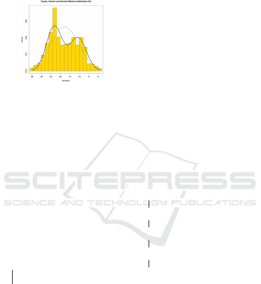
Figure 3: Toyota Normal Mixture and Normal distribu-

tion ﬁt s (black and grey respectively). Data source: Penta

Group.

3.8 Copula Model

In Algorithm 1, the symbols used are: Reputation

time series R, Lag L, r e quired simulation length n.

The internal variables are the auto-correlation matrix

A, a multi- variate Nor mal copula C, uniformly dis-

tributed marginal distributions of C G

, i = 1...n, Nor-

mal Mixture-distributed marginals Y

, i = 1...n , and

their corresponding auto-correlation p-values α

, i =

1...n. The process uses a procedure FIT(D) to ﬁt a

distribution D (in this case D is a Norm al Mixture ), a

function MVN (from the R package mvtnorm) to ini-

tialise a multi-variate normal copula , a fu nction AC to

test the marginal effect o f the simulate d data on the

autocorrelation of the input data, and a Loess smooth-

ing function LO.

Data: R, L, n

Result: Simulation of length n

Calculate best ﬁt parameters p = FIT (R(D));

Derive auto-correlation matrix A(R);

Initialise copula: C = MV N(A);

Generate uniform marginals G = Φ(C);

for i in 1:L do

= LO(Φ

−1

, p)) (NMix marginals) ;

Test auto-correlation: α

= AC(R,Y

);

end

Select optimal auto-correlation: α

opt

;

Return {Y

opt

, α};

Algorithm 1: Copula simulation.

3.9 ARIMA Model

The ARIMA modelling incorporates both auto-

regressive (AR) and moving average (MA) compo-

nents, although we suspect that the AR components

are much more important. With AR, MA and differ-

encing parameters p, q and d respectively, plus a con -

stant µ, λ and error term ε

, the ARIMA model used is

given in 9. The values of p, q and d ar e determine d us-

ing the auto-ARIMA method of Hyndman and Kh an-

dakar (Hyn dman and Khandak a r, 2008). Parameter

d is determ ined by carrying out successive unit-root

tests (D. Kwia tkowski and Shin, 1992) until a station-

ary series results. There is a correction for seasonal

data, although we would not expect reputation data to

exhibit any degree of seasonality since repu tation is

event-driven. Parameters p and q are determined by a

stepwise algorithm in which target values of p and q

are tested against for minimal AIC.

= µ + λ

∑

i=1

t−i

∑

i=1

t−i

+ ε

(9)

Having determined the parameter values, the

ARIMA ﬁt is done using maximum likelihood via

a state-space rep resentation of the ARIMA process.

The innovations and their variances are fou nd by a

Kalman ﬁlter (Gardner et al., 1980). In the ARIMA

algorithm below, the auto-AR IMA function used to

determine the ARIMA param eters (H yndman and

Khandakar, 2008) is de noted by FC(R), and the sim -

ulation function is denoted by FSim(R , . . . ).

Data: R, L, n

Result: Simulation with length n

Extract ARIMA order {p, d, q} = FC(R);

if (p > 0 & d > 0) then

ARMA: Y = FS (R , p, q);

end

if (p > 0 & d = 0) then

AR: Y = FS(R, p);

end

if (p = 0 & d > 0) then

MA: Y = FS(R, q);

end

if (p = 0 & d = 0) then

White noise: Y = FS(R, 0, 0, 0);

end

Return(Y)

Algorithm 2: ARIMA simulation.

In practice w e have never encountered the White

noise case.

3.10 Cholesky Model

Cholesky decomposition is an established way to de-

rive data that is correlate d with a given data set. The

autocorrelation matrix, derived from the observed

data forms the basis of the Cholesky decomposition.

As such, the correlation matrix A must be positive

DATA 2024 - 13th International Conference on Data Science, Technology and Applications

deﬁnite. That is, it must be symmetric with posi-

tive eigenvalues. A proof may be found in, for ex-

ample, (Golub and van L oan, 1 992) (Section 4.2.7).

Further details, including points arising from numer-

ical calculations, and supporting literature may be

found in (Higham, 1990 ). Appendix A shows how

this result app lies to auto-cor relation matrices. We

have found em pirically that, in all cases exam ined,

a Cholesky decom position is successful ( i.e. all au-

tocorrelation matrices encounte red are positive deﬁ-

nite). Consequently we have not ne eded to provide for

non-positive deﬁnite autocorrelation matrices. There

is a work -aroun d for that p ossibility. (Reb onato and

Jaeckel, 200 0) describe two methods to cast a non-

positive deﬁnite matrix into a positive deﬁnite state:

hypersphere decomposition and spectral decomposi-

tion.

A Cholesky decomposition pre sents problems in

the context of autocorrelation. First, the ’base’

Cholesky r e sult is a m atrix that has the same num-

ber of columns as the correlation matrix used to de-

rive it. Effectively, in our context wh ere many auto-

correlation components are close to 1, e ach column

is an almost carbon copy of th e orig inal data. The

problem then is to ﬁnd a r e asonable way to derive

a single simulation from those columns. To address

this problem for an auto-c orrelation matrix A of di-

mension L × L, assuming that a simulation of length

n is required, L vectors eac h of length n are gener-

ated f rom a probability distribution D (NMix in the

case of reputation data). The calculated Cholesky ma-

trix is applied to a matrix of the D-distributed vectors,

thereby ge nerating L correlated vectors. Each corre-

lated vector is assessed using the autoco rrelation test

(Section 3.6), and the optimal vector (given by maxi-

mum p-value in the auto-correlation t-test) is selected

as the simulation.

Data: R, L, n

Result: Simulation, with len gth n

Calculate best ﬁt parameters p = FIT (R(D));

Generate random samples Z = G(L, D, n);

Smooth samples Z = LO(Z);

Derive auto-correlation matrix A(R);

Cholesky decomposition : C

′

= Chol(A);

Generate correlated samples Y = XC

′

;

for i in 1:L do

Test auto-correlation: α

= AC(R,Y

);

end

Select optimal autoc orrelation

opt

= max (α

(pva l));

Select optimal sample vector Y

opt

;

Return {Y

opt

, α

opt

};

Algorithm 3: Cholesky simulation.

In Algorith m 2, the symbols u sed a re the same as

in Algorithm 1: Reputation time series R, Lag L, re-

quired simulation length n. Chol(A) is a function that

calculates the Cholesky decomposition of a matrix A.

In addition, G(L, D, n) is a function that generates L

random samples, each of length n, and each with Nor-

mal Mixture distribution D.

4 RESULTS

4.1 Prediction Accuracy

The ﬁrst set of results is a co mparison of actual and

predicted reputations. The starting point for these re-

sults is a partition of the available data in to a training

set (the ﬁrst 75%: da ys 1 to 547) and a test set (the

remaining 25%: days 548 to 730). Projections be-

yond 730 days were no t used. Predictions were made

using the training data only, and the essential details

of the conﬁgur ed models were noted. For the ARIMA

model, the only necessary c omponent was the ARIMA

ﬁt obje ct, c a lc ulated using the auto .arima function in

the R forecast package. The corresponding Cholesky

objects were the Cholesky decomposition ma trix and

the ﬁtted Normal Mixture parame te rs. For the Copula

model, the Copula correlation matrix and the ﬁtted

Normal Mixture parameters were needed. Predictio ns

were then made using th e test data with the objects

derived in the training ph ase.

Treated in this way, the train/test environments

provide a measure of the accuracy o f the test predic-

tion compared to the training prediction, via the mean

absolute error (MAE) for both. To that effect, the pro-

portion ate cha nge in MAE, ∆

(MAE)

, was calculated for

each target o rganisation (Equation 10).

∆

(MAE)

MAE

(train)

− MAE

(test)

MAE

(train)

(10)

The distribution of values of ∆

(MAE)

then gives an

indication o f gross deviations of MAE between the

training and test environments, for every organisation

considered . Figure 4 shows a plot of ∆

(MAE)

(on the

horizontal axis) against quantile (on the vertical axis).

The value ∆

(MAE)

= 1 represents a 100% increase in

MAE for the test environment relative to the training

environment. The corresponding low quantile values

shows that in the majority of cases, an order of m a g-

nitude difference, which would indicate instability in

a model, is absent. Only one value of ∆

(MAE)

out of

125 exceeded the nominal order of magnitude limit:

14.19 using the Cholesky model. A second instance

of the Cholesky model had a ∆

(MAE)

value o f 9.63:

just below the limit. The largest ∆

(MAE)

values for

Reputation, Sentiment, Time Series and Prediction

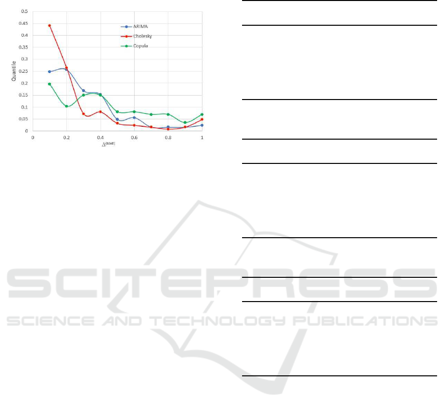
the ARIMA and Copula models were 1.17 and 3.82

respectively.

Figure 4: Comparison of MAE in training and test environ-

ments.

4.2 Auto-Correlation Results

The principal results of this analysis are presented in

this section. The a uto-correlation test (Section 3.6)

for the three predic tion methods (sections 3.8, 3.9 and

3.10) are shown at two signiﬁcance levels: 5% and

1%. U sin g ﬁve runs in each case, Tables 1, 2 and 3

show the mea ns and stand a rd deviations of the num-

ber of organisation that ’passed’ the auto-c orrelation

test. A ’pass’ is a p-value greater than 0.05 for 5%

signiﬁcance and greater than 0.01 for 1% signiﬁcance.

Column heading ’Simulation length’ refers to the per-

centage augmentation of o bserved data by simulated

data.

The auto-correlation results for the th ree predic-

tion methods are consistent in th at the ’success’ rate

reduces as the pre diction length increases. Of the

three, Cholesky provides optimal ’succe ss’. There

are indications, particularly from the Cholesky results,

that the ’success’ rate levels off for large prediction

lengths. It is likely that this effect is due to converg-

ing r e semblance of the predicted data structure to the

observed data structure.

4.3 Simulation Illustrations

This section contains examples of the three simula-

tion mod es, to which we add qualitative comments on

the characte ristics of the simulations. In ea ch case,

the observed data is shown in red, the three simu-

lations are shown in green, and th e median simu la-

tion is shown in blue. The illustrations are for Mi-

crosoft, which has a typical reputation proﬁle of many

large corporates, subject to the gen eral sentiment level

(positive, negative or neutral). Microsoft’s sentimen t

is mostly positive, and has the characteristic ’jagged’

Table 1: Augmentation of observed data by simulated data:

Copula method.

Simulation Mean SD

length 5% 1% 5% 1%

5% 0.979 1.000 0.004 0.000

10% 0.779 0.90 6 0.004 0.007

15% 0.672 0.76 0 0.018 0.009

20% 0.587 0.70 2 0.012 0.009

25% 0.541 0.60 3 0.017 0.004

33% 0.448 0.54 4 0.016 0.006

Table 2: Augmentation of observed data by simulated data:

ARIMA method.

Simulation Mean SD

length 5% 1% 5% 1%

5% 0.950 0.990 0.009 0.000

10% 0.794 0.89 6 0.018 0.019

15% 0.623 0.75 5 0.030 0.013

20% 0.557 0.70 1 0.036 0.022

25% 0.541 0.66 3 0.025 0.032

33% 0.475 0.59 2 0.018 0.033

Table 3: Augmentation of observed data by simulated data:

Cholesky method.

Simulation Mean SD

length 5% 1% 5% 1%

5% 0.981 1.000 0.007 0.000

10% 0.837 0.93 3 0.017 0.012

15% 0.722 0.81 0 0.015 0.019

20% 0.712 0.80 0 0.032 0.017

25% 0.667 0.73 9 0.022 0.026

33% 0.662 0.71 7 0.046 0.040

reversing pattern with prolonged upward and down-

ward movements. The two year proﬁle is shown in

Figure 5, for which the sen timent mean and standard

deviation were 10.76 an d 8.10 respectively. The end

of the observed data period is marked at day 730. For

each simu lation type illustrated, the simulation is f or

110 days: 15% more than the length of th e observed

data. Only the latest six months of the observed data

are shown, in ord er to better highlight the proﬁle of

each simulation .

5 DISCUSSION

The numerical results in Section 4 invite a choice

of which prediction method to use. Table 3 in-

dicates that Cholesky decomposition is the optimal

method, since it provides a higher proportion of auto-

DATA 2024 - 13th International Conference on Data Science, Technology and Applications

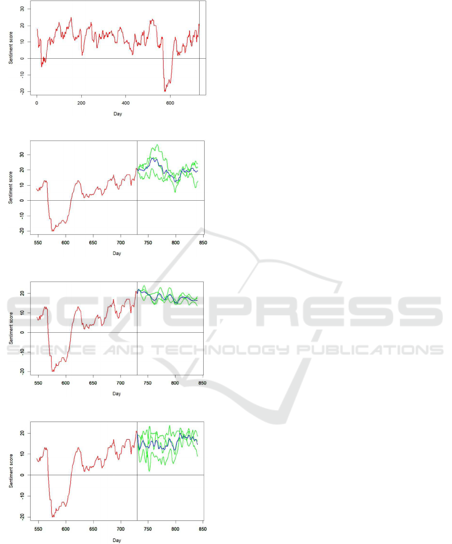
Figure 5: Microsoft: Microsoft observed data.

Figure 6: Microsoft: three ARIMA simulations.

Figure 7: Microsoft: three Copula simulations.

Figure 8: Microsoft: three Cholesky simulations.

correlation ’successes’. The Cholesky choice would

be clear, were it not for a qualitative examination of

the predicted data, and of its microstructur e. Figure

8 shows that the day-to-day variation in the predic-

tion is greate r than the day-to-day variation for the

ARIMA a nd Copula methods. Fur ther, the predictions

for ARIMA and Copula appear, subjectively, to be less

volatile than the observed data. Examination of sim-

ilar plots for other organisations conﬁrms that view.

We have investigated, albeit brieﬂy, a way to reduce

the volatility of the Cholesky prediction. A scale fac-

tor can be derived as a function of prediction resid-

uals resulting from a piecewise lin e ar ﬁt to the ob-

served data. The same technique can also be used

to increase the volatility of the ARIMA and Cop ula

predictions. Despite some misgivings, we prefer the

Cholesky method because of its superior conformance

to the o bserved data auto -correlation.

Normally we would not recommend calculating

predictions that extend far beyond the bounds of the

observed data. A 10-15% extension would be an up-

per limit. We have exten ded further in this analy-

sis to illustra te the limitations and capabilities o f the

overall method. The further extensions h ave revealed

a slow convergence to what appears to be a limit-

ing value for the percentage ’success’ metric. Con-

vergence is attributable to convergence of the auto-

correlation structure s of the observed data and the pre-

diction.

Investigating the pr edictive nature of rep utation is

important because it has implications for risk man-

agement and corporate decision- making. As part of

a generalised risk mitigation process (which nearly

always focuses primarily on mone ta ry risk), estimat-

ing risk due to reputation can provide insights which

balance sheet items cannot. For examp le , a predicted

downturn in reputation could signa l future difﬁculties

in selling products or in hiring staff. Mor e generally,

tracking r eputation following th e introduction of new

products can indicate wheth er or not it is worth in-

troducing similar products at a later stage. The q ues-

tion of m onetary valuation of rep utation was tackled

in (Mitic, 2024), in which reputation was valued in

terms of share price. Share capitalisations for large

corporates are often valued in hun dreds of millions of

euros, which is not useful for insights into individual

products. However, if a company tracks sales with

reputation, the possibility of monetising reputa tion in

terms of sales becomes realistic. Thereafter, reputa-

tion predictio n can be used to predict sales. Further

research is re quired on this topic, but it would proba-

bly have to rem ain in the domain of in dividual com-

panies who can track their own sales on a daily basis.

5.1 Further Work

In addition to monetisation of reputation in terms of

product sales (as discussed a bove), prediction using

statistical prop e rties of reputation time series pre sents

Reputation, Sentiment, Time Series and Prediction

possibilities. In pa rticular, neural networks using

Long Short Term Memory (LSTM) is a fruitf ul area

because LSTM can mimic the “choppiness“ of repu-

tation time series due to its mechanism for selectively

retaining or discard ing information using input gates

and forget gates respectively. However, this type of

neural network is very slow to train. Recent work

on this topic in other contexts includes (Yadev and

Thakkar, 20 24). Adding attention layers to a neural

network may also be a way forward, provided that the

attention can be directed at particular features of the

data. A recent study (Wen and Li, 2023) in the con-

texts of air quality, electricity and share price is en-

courag ing.

ACKNOWLEDGEMENTS

We acknowledge the c ontinuing support and assis-

tance of the staff of Penta Group.

REFERENCES

Cambridge (2023). Cambridge Di ct ionary online. CUP

https://dictionary.cambridge.org/ dictionary/english/.

Carreras, E., Alloza, A., and Carreras, A. (2013). Corporate

Reputation. LID Publishing, London, 1st edition.

Cole, S. (2012). The impact of reputation on market value.

In World Economics 13(3), pp. 47-68. https://www.

world-economics-j ournal.com/P apers/Using-Reputat

ion-to-Grow-Corporate-Value.aspx?ID=563.

D. Kwiatkowski, P.C. Phillips, P. S. and Shin, Y. ( 1992).

Testing the null hypothesis of stationarity against the

alternative of a unit root. In Jnl. Econometrics 54 pp.

159-178.

Das, S. and Chen, M. (2007). Yahoo! for ama-

zon: Sentiment extraction from small talk on the

web. In Management Science 53(9) pp. 1375-1388.

http://www.icefr.org/icefr2021.html.

Durant, H. (1954). The gallup poll and some of its

problems. In The I ncorporated Statistician 5(2) pp.

101–112. https://www.jstor.org/stable/2986465.

Fombrun, C., Gardberg, N. A., and Sever, J. M. (2000).

A multi - stakeholder measure of corporate reputation.

In Journal of Brand Management 7(4) pp. 241–255.

https://link.springer.com/article/10.1057/bm.2000.10.

Fombrun, C., Ponzi, L. J., and Newburry, W. (2015).

Stakeholder tracking and analysis: the reptrak

system for measuring corporate reputation. I n

Corporate Reputation Review 18(1), pp. 3-24.

https://link.springer.com/article/10.1057/crr.2014.21.

Gallup, G. and Rae, S. (1968). The Pulse of Democracy:the

public-opinion poll and how it works. Simon and

Schuster, New York, 1st edition.

Gardner, G., Harvey, A., and Phillips, G. (1980). Algorithm

AS 154: An algorithm for exact maximum likelihood

estimation of autoregressive-moving average models

by means of kalman ﬁltering. In Applied Statistics 29

pp. 311-322. 10.2307/2346910.

Golub, G. and van Loan, C. (1992). Matrix Computations.

Johns Hopkins University Press, Baltimore, 1st edi-

tion.

Higham, N. (1990). Analysis of the cholesky decom-

position of a semi-deﬁnite matrix. In Reliable Nu-

merical Computation (eds. M. G. Cox and S. J.

Hammarling), pp. 161–185. Oxford University Press,

10.2307/2346910.

Hyndman, R. and Khandakar, Y. (2008). Automatic

time series forecasting: The forecast package for

R. In Jnl. Statistical Software, 26(3) pp. 1-22.

doi:10.18637/jss.v027.i03.

Jacobs, L. and Shapiro, R. (1995). Presidential

manipulation of polls and public opinion. In

Political Science Quarterly 110(4) pp. 519-538.

doi:10.2307/21518825.

Janson, J. ( 2014). The Reputation Playbook. Harriman

House, Petersﬁeld, UK, 1st edition.

Lippman, W. (1922). Public opinion. Harcourt, Brace

and Company, available from Project Gutenberg at

https://gutenberg.org/ebooks/6456.

Liu, B. (2015). Sentiment Analysis: Mining Opinions, Sen-

timents and Emotions. CUP, New York, 1st edition.

Loke, R. and K achaniuk, D. (2020). Sentiment polar-

ity classiﬁcation of corporate review data with a

bidirectional long-short term memory (bilstm) neu-

ral network architecture. In Proc, 9th Interna-

tional Conference on Data Science, Technology and

Applications (DATA 2020), pp 310-317. ScitePress

doi:10.5220/0009892303100317.

Loke, R. and Kisoen, Z. ( 2022). The role of fake review

detection in managing online corporate reputation. In

Proc, 11th International Conference on Data Science,

Technology and Applications (DATA 2022), pp 245-

256. ScitePress doi:10.5220/0011144600003269.

Loke, R. and Reitter, W. (2021). Aspect based sen-

timent analysis on online review data to predict

corporate reputation. In Proc, 10th International

Conference on Data Science, Technology and Ap-

plications (DATA 2021), pp 343-352. ScitePress

doi:10.5220/0010607203430352.

Loke, R. and Vergeer, J. (2022). Exploring corporate repu-

tation based on sentiment polarities that are related to

opinions in dutch online reviews. In Proc, 11th Inter-

national Conference on Data Science, Technology and

Applications (DATA 2022), pp 423-431. ScitePress

doi:10.5220/0011285500003269.

Mitic, P. (2015). Improved goodness-of-ﬁt tests for opera-

tional risk. In Journal of Operational Risk, 15(1), pp

77-126. Incisive Media doi:10.21314/JOP.2015.159.

Mitic, P. (2024). What is the value of reputation? In Proc.

ICICT 2024, London. To appear in Springer L NCS.

Rebonato, R. and Jaeckel, P. ( 2000). The most general

methodology for creating a valid correlation matrix

for risk management and option pricing purposes.

In Journal of Risk, 2(2), pp 17-27. I ncisive Media

doi:10.21314/JOR.2000.023.

DATA 2024 - 13th International Conference on Data Science, Technology and Applications

Reichheld, F. F. (2003). The one number you need

to grow. In Harvard Business Review 81(12)

pp. 46–54. https://hbr.org/2003/12/the-one-number-

you-need-to-grow.

Renner, M. (2011). Generating Trust via C orporate Repu-

tation. Wissenschaftlicher Verlag, Berlin, 1st edition.

Royston, P. (1992). Approximating the shapiro–wilk w-test

for non-normality. In Statistics and Computing 2(3),

pp. 117–119. doi:10.1007/BF01891203.

Rozin, P. and Royzman, E. B. (2001). Negativity bias,

negativity dominance, and contagion. In Personal-

ity and Social Psychology Review. 5(4) pp. 296–320.

doi:10.1207/S15327957PSPR0504

Russell, R. (2023). The future of Corpo-

rate Communications. Edelman.com,

https://www.edelman.com/2023-future-of-corporate-

comms.

Shapiro, S. S. and Wilk, M. B. (1965). An analy-

sis of variance test for normality (complete sam-

ples). In Biometrika, 52(3,4), pp. 591-611.

doi:org/10.2307/2333709.

SignalAI (2024). Signal AI Sharpens Reputation and Risk

Capabilities with Acquisition of Social 360. Press Re-

lease, https://signal-ai.com/press release/social-360/.

Weber-Shandwick (2020). The State of Corporate Reputa-

tion in 2020: Everything Matters Now. Weber Shand-

wick, https://we bershandwick.com/n ews/the-state-o

f-corporate-reputation-in-2020-everything-matters-n

ow.

Wen, X. and Li, W. (2023). Time series pre-

diction based on lstm-attention-lstm model.

In IEEE Access 11, pp.48322-48331.

https://doi.org/10.1109/ACCESS.2023.3276628.

Yadev, H. and Thakkar, A. (2024). Noa-lstm: An efﬁcient

lstm cell architecture for time seri es forecasting. In

Expert Systems with Applications 238, pp. 122333.

https://doi.org/10.1016/j.eswa.2023.122333.

Zendesk (2013). Customer service and Business results: a

survey of customer service from mid-size Companies.

Zendesk.com, http://cdn.z endesk.com/resources/wh

itepapersZendesk\

WP\ Customer\ Service//\ and

Business\ Results.pdf.

APPENDIX A

Proposition.

An auto -correlation matrix A is positive deﬁnite

(ζ

′

Aζ > 0 for all vectors ζ) , and therefore admits a

Cholesky decomposition.

Preliminary Result.

A positive deﬁnite m a trix has a Cholesky deco mposi-

tion (Golub and van Loan, 199 2) (Section 4.2.7)

Proof.

Let A be an L × L auto-correlation matrix and let its

column vectors be z = {z

, z

, . . . z

}. Symmetry is

assured for (auto-)c orrelation matrices since for any

two vectors z

and z

, cor(z

, z

) = cor(z

, z

); i, j =

1 . . . L.

By deﬁnition, A = E[(z − ¯z)(z − ¯z)

′

]. Then, for all

vectors ζ,

′

Aζ = ζ

′

E[(z − ¯z)(z − ¯z)

′

]ζ

= E[ζ

′

(z − ¯z)(z − ¯z)

′

ζ]

= E[yy

′

] where y = ζ

′

(z − ¯z)

= E[var(y)] > 0 ∀y > 0 (11)

Also A is symmetric, and therefor e A is positive

deﬁnite.

Reputation, Sentiment, Time Series and Prediction