Is Positive Sentiment Missing in Corporate Reputation?
Peter Mitic
a
Department of Computer Science, UCL, London, U.K.
Keywords:
State-Space, Kalman Filter, Kalman, Forward Filtering Backward Sampling, FFBS, MCMC, TNA,
Reputation, Sentiment, Missing Sentiment, Missing Positive Sentiment, Negative Bias.
Abstract:
The value of a perceived negative bias is quantified in the context of corporate reputation time series, derived
by exhaustive data mining and automated natural language processing. Two methods of analysis are proposed:
State-Space using a Kalman filter time series with a Normal distribution profile, and Forward Filtering Back-
ward Sampling for those without. Normality tests indicate that approximately 92% of corporate reputation
time series do fit the Normal profile. The results indicate that observed positive reputation profiles should
be boosted by approximately 4% to account for negative bias. Examination of the observed balance between
negative and positive sentiment in reputation time series indicates dependence on the sentiment calculation
method, and region. Positive sentiment predominates in the US, Japan and parts of Western Europe, but not in
the UK or in Hong Kong/China.
1 INTRODUCTION
Measuring sentiment and opinion using Natural Lan-
guage Processing (NLP) has been an established pro-
cedure since work on Phase-Structure Grammar in
the 1950s (Chomsky, 1957). Translation of natural
language sentences into a format that can be used by
computers remains the basis of NLP today, including
the recent Large Language Models (OpenAI, 2019).
This paper concerns a particular aspect of the ac-
curacy of sentiment measures, embedded in a much
wider framework: reputation. That aspect is ”miss-
ing positive sentiment”, which is closely related to the
idea of negative bias. Our proposition is that negative
bias exists in the context of reports on corporate af-
fairs, and is due to unexpressed positive content.
Written statements about particular organisations
can be positive (as exemplified by words such as
”good” or ”improved”), or they can be negative (us-
ing words such as ”poor” or ”bad”). The underly-
ing idea of this paper is the possibility that there is a
proportion of positive statement that is not expressed,
possibly because of a lack of emotion associated with
positivity. The analysis presented aims to detect and
quantify the extent of unexpressed content. In doing
so, the overall balance between positive and negative
sentiment is noted.
a
https://orcid.org/0000-0002-9845-4435
1.1 Structure of this Paper
The paper is divided into the following sections.
1. This introduction, including a statement of the
problem to be solved (Section 1).
2. An example of reputation, expressed as a time se-
ries (Section 1.2.1)
3. Related literature (Section 2)
4. Methods used (Section 3)
5. Results (Section 4)
6. Discussion and issues arising (Section 5)
The core of the Methods section is to first assess the
positive/negative balance for reputation time series
using observed reputation time series. Then, assum-
ing that some positive sentiment is ”missing”, we at-
tempt to measure its extent by using State-Space anal-
yses. The purpose is to reveal an underlying relatively
noise-free ’hidden’ reputation time series, from which
it is possible to estimate the missing positive com-
ponent of that reputation. An alternative procedure
which is more widely-applicable but is slower to cal-
culate is proposed for validation of the result.
Mitic, P.
Is Positive Sentiment Missing in Corporate Reputation?.
DOI: 10.5220/0012763100003756
Paper published under CC license (CC BY-NC-ND 4.0)
In Proceedings of the 13th Inter national Conference on Data Science, Technology and Applications (DATA 2024), pages 71-81
ISBN: 978-989-758-707-8; ISSN: 2184-285X
Proceedings Copyright © 2024 by SCITEPRESS – Science and Technology Publications, Lda.
71

1.2 Reputation and Sentiment: A Brief
Overview
The analysis in this paper is heavily dependent on
time series and statistical concepts, so it is impor-
tant to formulate the term ”reputation” in terms that
fit the necessary paradigms. To do that, we separate
the terms ”reputation” and ”sentiment”. The latter is
well-defined in the context of NLP (for example by
(Liu, 2015)), but the former is a relatively new con-
cept. Consequently, both are defined in a formal way
in Section 3.1. Additionally, the term ”opinion” is
also defined.
Details of the reputation measurement process
used to derive the data used in this study can be found
in (Mitic, 2017). Compiling a daily reputation time
series comprises the following stages, targeted upon a
particular organisation, T.
1. Exhaustive data mining of textual records. Text
is derived by setting up dedicated data feeds to
both social and ’traditional’ media sources. Ex-
amples of ’traditional’ media include radio and
TV news channels (e.g. BBC, Sky TV, Fox
Media), newspapers (e.g. the Financial Times,
Wall Street Journal), financial organisations (e.g.
Bloomberg, Reuters), and consumer reviews (e.g.
from Google, Amazon). Social media sources in-
clude X (”Twitter”), Facebook and WhatsApp.
2. NLP to derive sentiment per record.
3. Averaging sentiments received on each day,
weighted by importance/significance. This is the
’observed’ sentiment for day t, denoted by y
t
in
this paper).
4. Conditioning y
t
to remove ’noise’.
5. Forming a time series {y
t
},t = 1,2,... , which is
the ’reputation’ of T
1.2.1 Reputation Examples
To crystallise the ideas of casting reputation as a time
series, and to illustrate the essential characteristics
of those time series, Figures 1, 2 and 3 show recent
views of typical reputation profiles: Lego, NASA and
Singapore Airlines. Each plot shows the sentiment
score y
t
on the vertical axis on a scale of -100 to +100,
for each of 730 days on the horizontal axis. The hori-
zontal line at y
t
= 0 sentiment indicates entirely neu-
tral sentiment. The portions of the plot above that line
indicate positivity (for example, for increased prof-
its recorded on financial statements), whereas the por-
tions of the plot below indicate negativity (for exam-
ple, for negative customer experience). The plots in-
clude Loess-generated smoothed profiles, and Loess-
generated trend curves.
Many reputation plots express mostly positive
sentiment (illustrated by Lego) or mostly negative
sentiment (illustrated by NASA). Plots that straddle
the positive/negative border with a high frequency os-
cillation, similar to that of Singapore Airlines, are less
common. Together, the three plots illustrate features
typical of all reputation time series, listed below.
• A macro-structure of peaks and troughs, with lit-
tle discernable periodic effect or length (in time)
between successive peaks and troughs.
• Large upward or downward moves over short time
periods. The NASA plot has several.
• Small day-to-day variation, representing ’noise’.
• Isolated ’shocks’: extreme (usually negative) sen-
timent lasting one or two days, often due to mul-
tiple reports of the same adverse event. Several
are shown on the Lego plot. Negative ’shocks’ are
more common than positive ’shocks’.
• Sentiment concentration principally within a
broad range (-50,50). Very few instances of sen-
timent outside this range are encountered. This
concentration is most likely due to averaging pro-
cesses in NLP calculations.
Figure 1: Lego (daily) reputation (in red) July 2021-June
2023. Blue line: smoothed sentiments; green line: trend.
Data source: Penta Group.
2 RELATED WORK
In this review, we concentrate specifically on one par-
ticular aspect which is of relevance to our study. That
is the excess of negative sentiment compared to posi-
tive sentiment in instances of daily accumulation and
analysis of sentiment. Most research has concentrated
on the detection and analysis of sentiment bias which
we regard as a precursor for the existence of excess
negative sentiment. For example, (Rozin and Royz-
man, 2001) offer a full discussion of sentiment bias,
DATA 2024 - 13th International Conference on Data Science, Technology and Applications
72

Figure 2: NASA (daily) reputation (in red) July 2021-June
2023. Blue line: smoothed sentiments; green line: trend.
Data source: Penta Group.
Figure 3: Singapore Airlines (daily) reputation (in red) July
2021-June 2023. Blue line: smoothed sentiments; green
line: trend. Data source: Penta Group.
and initiated the term ’negative bias’. Here we con-
sider research on the value of excess negative senti-
ment.
Direct evidence comes from (Zendesk, 2013) in a
study of responses to customer service. They found
that people are more likely to express negative ex-
periences rather than positive. Consequently, there
is an excess volume of negative sentiment. Specif-
ically they report that 95% of users were likely to
share a negative experience, as opposed to 87% per-
cent for a positive experience. Some reasons for these
findings are suggested. First, negative comments are
driven by emotional responses, which last longer in
the mind and appear more urgent than positive com-
ments. Second, for the same reason, negative com-
ments are given unprompted, whereas positive com-
ments often have to be solicited. It is tentatively sug-
gested that customers take more note of negative com-
ments, and are more likely to post negatives in order
to warn other customers.
(Finkelstein and Fishbach, 2012) suggest that a
potential reason for an excess of negative feedback
is that there is a difference in responses from novices
and experts. Novices seek and provide positive feed-
back in order to make decisions, whereas experts are
more likely to provide negative feedback because pos-
itive sentiment is what they already know. Since there
are fewer novices, negative feedback prevails.
The study by (Moe and Schweidel, 2012) (and
summarised in (Moe and Schweidel, 2013)) indicates
an excess of negative comments due to different be-
haviour modes for less active and more active people
who posted online comments. They consider that on-
line opinions are dominated by ’activists’ who offer
negative opinions, and skew sentiment negatively.
(Tsugawa and Ohsaki, 2017) investigated the re-
lationship between message sentiment on social me-
dia and the volume and speed of message diffu-
sion. They analysed 4.1 million tweets and their
retweets, and found that the reposting volume of neg-
ative messages was 20–60% higher than that of pos-
itive and neutral messages. The result is reinforced
by (Ferrara and Yang, 2015), who found that nega-
tive messages spread faster on social media than posi-
tive ones. However, positive messages reached larger
audiences. Their dataset, which was not a random
selection, comprised approximately 36% of positive
tweets, 22% of negative tweets, with 42% neutral.
The opposite effect is reported by (Stieglitz and Dang-
Xuan, 2013), who found, in the context of tweets, no
evidence of sentiment bias.
Two later studies investigated the incidence of
positive and negative sentiment on social media.
(Bellovary and Goldenberg, 2021) investigated the
spread speed of online sentiment. Overall, negativ-
ity was about 15% more prevalent than positivity, and
more users responded to negative tweets than did to
positive tweets. This result is particularly insightful
in the context of reputational analysis. A major (data-
mined) source of reputational data is news reports,
for which, the authors found, negativity is more fre-
quent and more impactful than positivity. (Antypas
and Camacho-Collados, 2023) reached a similar con-
clusion.
An example of intrinsic negative bias is (arguably)
the Net Promoter Score - NPS
1
(Reichheld, 2003),
which is a very simple scoring system based on sub-
jective answers to a single question: On a scale of 0-
10, how likely are you to recommend this company to
a friend or colleague?. The NPS is then the difference
between the percentage of 9-10 (promoter) scores and
the percentage of 0-6 scores (detractors). Scores 7 and
8 are regarded as ”passive”. The numerical imbalance
induces negative bias.
Overall, previous research indicates evidence of
an excess of negative sentiment, particularly on social
media. This result prompts us to consider whether or
not some positive sentiment is ”missing” from repu-
tation time series. The main reason is the emotional
1
Published by Bain and Co., https://www.bain.com/
Is Positive Sentiment Missing in Corporate Reputation?
73

response triggered preferentially by negative feelings,
as surmised in (Zendesk, 2013). We present our own
findings on this topic in section 4.1.
2.1 Positive Bias
Few indications of positive bias are available in the
context of products or organisations. (Park and Rhim,
2018) studied online chat satisfaction surveys, and
concluded that a majority of non-respondents were
likely to be dissatisfied with the chat service. How-
ever, a majority of respondents had positive opinions.
That result agrees with earlier work on Amazon On-
line product reviews by (Hu and Zhang, 2007). Re-
views, expressed as ”star ratings” were significantly
more positive (4* and 5*) than negative (1* and 2*)
for books, DVDs and videos.
Closely related to positive bias is the concept of
Confirmation bias. (Powell and Holyoak, 2017) pro-
vide confirmation bias examples in which people pre-
ferred a product with more reviews to one with fewer
reviews, even though their statistical model indicated
that the latter was likely to be of higher quality than
the former.
3 METHODS
A brief investigation of negative/positive sentiment
balance is outlined. All of the following sub-sections
deal with finding how ”missing positive sentiment”
might be quantified, assuming that it is present.
3.1 Definitions
In this section we give a brief definition of Opinion,
Sentiment and Reputation. There are indications of
the necessary definitions in, for example, (Loke and
Vergeer, 2022) in phrases such as ”collective view”
and ”built over time”. The general idea of the scope of
reputation is summarised in (Loke and Kisoen, 2022):
”a summary of internal and external perceptions of an
organisation”. We argue that reputation should extend
much further. Specifically, it should include broad-
casting, news reports, company statements and social
media.
(Liu, 2015) defines Opinion as a function or
algorithm F of a comment X in text form, provided
by a Holder H, aimed at a target organisation T with
influence U ∈ (0,1), and given at a time t (nominally
one day). F maps X to a subset of the real numbers
[−r,r];r ∈ R
+
. This defines a numeric ”score” for
textual content. Sentiment, S, is a set of opinions
expressed by n
h
holders, in n
x
texts, on the same
target T, all at the same time, using a function Ψ
which forms a weighted average of the opinion hold-
ers using their influences. The idea that Sentiment
should refer to a set of Opinions is unusual, and
differs from the view expressed in (Liu, 2015), where
in the context of NLP, the distinction is not needed.
Reputation, y
t
(T ), is a time series of Sentiments over
an extended time period of length τ. For convenience,
we omit the target T in the equations in Section 3.
Definition: Opinion.
O
t
(X,H,T,U) = F (X | H,T,U) ∈ [−r,r] (1)
Definition: Sentiment.
S
t
(T ) = Ψ({O
t
(X
i
,H
j
,T,U
j
)});
i = 1..n
x
; j ∈ 1..n
h
(2)
Definition: Reputation.
y
t
(T ) = {S
t
(T )}; t = 1..τ (3)
3.2 Negative/Positive Sentiment
Analysis
We first undertake a simple analysis of the balance
between positive and negative sentiment in reputation
time series. Evidence from section 2 indicates that ex-
cess negative sentiment is prevalent in many contexts,
predominantly in social media. For each reputation
time series, the number of days on which positive,
neutral and negative sentiment was recorded, were
noted. In this context, three sentiment categories were
designated as in equation 4. In practice, the results
were insensitive to the ’neutral’ limit 2. There was
little variation in the results by extending the ’neutral’
limit to 5.





Positive: y
t
> 2; t = 1...τ
Neutral: −2 ≤ y
t
≤ 2 t = 1...τ
Negative: y
t
< −2 t = 1...τ
(4)
The results are shown in section 4.1.
3.3 Negative Bias Analysis
We now surmise that excess negative sentiment does
exist in reputational signals. To quantify it, for
any given corporate organisation, we use State-Space
analysis and the Kalman filter (Harvey, 1990) to ex-
tract the state (’hidden’) signal. The state signal pre-
serves the profile of the observed signal, but removes
some of the noise. That extraction also defines a vari-
ance component. Together, the estimate of the state
signal and its variance enable a high quantile of the
DATA 2024 - 13th International Conference on Data Science, Technology and Applications
74

estimated state to be calculated, and the difference
between the high quantile and the observed signal is
taken as the ’missing’ signal. So if y
t
represents the
observed sentiment on day t, x
t
and P
t
are the state
sentiment mean and variance respectively, then the
’missing’ sentiment on day t, m
t
, is given by the first
part of equation 5. The value of z represents either
95% or 99% (2-tailed) confidence. A single figure
measure of the ’missing positive sentiment’, M
z
, for
the organisation is the mean of all values of m
t
over a
day range 1...τ.
m
t
= x
t
+ z
√
P
t
M
z
= m
t
1 ≤ t ≤ τ (5)
3.4 Data
Reputation data is sourced from Penta Group
(https://pentagroup.co). Two data sets were extracted.
The first was used for the ”missing positive senti-
ment” analysis. We selected 261 corporate organisa-
tions representating the principal world industrial and
service sectors: energy, manufacturing, travel, edu-
cation, financial, media, food production, and retail.
The data range was two years: from Q3 2021 to Q3
2023, a total of 730 days. The observed data is pre-
sented on a continuous scale from -100 (worst possi-
ble sentiment) to +100 (best possible sentiment). Zero
(or very near to zero) represents neutral sentiment.
The second data set was used for the posi-
tive/negative sentiment balance analysis. Reputa-
tional time series for constituents of a range of major
stock indices were sourced, together with 40 reputa-
tional time series for organisation that are non stock-
exchange listed. The second selection is nearer to a
random sample than is the first.
Full details of both data sets are given in Sections
4.1 and 4.2.
3.5 Assumptions
• Measurements of the observed data must be inde-
pendent in order to estimate the values of x
t
and P
t
in the Kalman filter calculation (section 3.7). The
method of data collection ensures independence,
because components of the sentiment measure for
day t originates on day t only. The reputation
value therefore starts from zero on each day.
• The set of sentiments must be Normally dis-
tributed. This point is discussed in section 3.6.
The non-normal case is discussed in section 3.8.
3.6 Gaussian Data Requirement
The histograms of the two-year reputation data for
many organisations show that, informally, Normal
distributions might apply. All reputation data series
were tested for normality using the TNA test (Mitic,
2015), which is a generalisation of a Q-Q
2
plot, and
is insensitive to outliers, and to data set size. Apply-
ing the TNA test, the normality null hypothesis was
rejected in only 19 cases. The remaining 19 could be
’normalised’ by at least one of the following transfor-
mations.
• A log transformation, applied separately to posi-
tive and negative sentiment: y
t
[y
t
> 0] → log(y
t
);
y
t
[y
t
≤ 0] → −log(−y
t
)
• A square root transformation, applied separately
to positive and negative sentiment: y
t
[y
t
> 0] →
p
(y
t
); y
t
[y
t
≤ 0] → −
p
( −y
t
)
• A Box-Cox transformation, using the modifica-
tion by (Yeo and Johnson, 2000), which can ac-
commodate negative arguments. For positive α, λ
is selected to ’normalise’ by transforming
y
t
→
(x
λ
+α)−1
λ
;λ ̸= 0 and y
t
→ log(y
t
+ α); λ = 0.
• Removal of extreme outliers.
We use the State-Space method applied to unmodified
reputation data as the primary means of estimating
whether or not negative bias exists in the data. Data
transformations, as described, can be used to generate
normally distributed data, but may have contingent ef-
fects that are undesirable. In particular, proving that
State-Space analysis applied to transformed data has
precisely the same effect as for untransformed data
needs much more analysis. In Section 3.8 a Markov
Chain Monte Carlo (MCMC) method, applicable for
non-normal data, is discussed. The MCMC and State-
Space results are similar (Tables 4 and 5), but State-
Space analysis is much faster. We are therefore con-
tent to apply a State-Space analysis to unmodified
reputational data, and to use MCMC as a comparison.
3.7 State-Space Estimation: Outline
The sequence of equations in this sub-section follows
the exposition by (Shumway and Stoffer, 2016), as
does the R-code to implement it. We start with a rep-
utation time series {y
t
: 1 ≤t ≤ τ} measured in days
from 1 to τ. These are ’noisy’ observations of a ’hid-
den’ signal, which is less noisy. We aim to determine
a parallel series {x
t
} which represents the state of the
system: quantities that are not observed directly, but
2
Quantile-Quantile: a plot of empirical quantiles
against quantiles calculated using a theoretical distribution
Is Positive Sentiment Missing in Corporate Reputation?
75

can only be inferred via the actual observation. The
aim is to estimate an upper limit for the state vector
x
t
given the observations y
t
, and to attribute the dif-
ference between that upper state limit and the corre-
sponding observations as unobserved (or ’missing’)
positive sentiment.
We assume that x
t
and y
t
are related, in a general
case, as in equation 6. In those equations, w
t
and v
t
are stochastic errors, and are functions of matrices Q
and R, which describe the correlation structures of the
stochastic error associated with x
t
and y
t
respectively.
Φ is the correlation matrix for vector x
t
, and has to be
estimated from observations. The matrix A
t
is the ob-
servation matrix and represents a measurement scal-
ing. The time dependency of A
t
distinguishes a State-
Space process from a conventional linear model. The
vector u(t) is an exogenous vector, scaled by matrices
γ and Γ in the two cases.
x
t
= Φx
t−1
+ γu
t
+ w
t
; w
t
∼ N(0,Q); 1 ≤t ≤ τ
y
t
= A
t
x
t
+ Γu
t
+ v
t
; v
t
∼ N(0,R); 1 ≤t ≤ τ (6)
The State-Space exposition in (Shumway and
Stoffer, 2016) describes the development of estima-
tors ˆx
t
of the x
t
, with corresponding variance estima-
tors
ˆ
P
t
via the Kalman filter. The variance estimators
are used to calculate upper confidence limits that rep-
resent the ”missing positive sentiment”. The estima-
tors are, in general:
ˆx
t
=

x
t
|y
y

1 ≤ t ≤ τ
ˆ
P
t
=

(x
t
− ˆx
t
)(x
t
− ˆx
t
)
′

1 ≤ t ≤ τ (7)
The Kalman filter provides a way to update the
state vector x
t
from the previous state vector x
t−1
plus
a new observation y
t
without having to reprocess all
previous observations. The update equations take the
form in equation 8, in which K
t
is the Kalman gain.





K
t
= P
t−1
A
′
t
(A
t
P
t−1
A
′
t
+ R)
−1
x
t
= x
t−1
+ K
t
(y
t
−A
t
x
t−1
−Γu
t
)
P
t
= (I −K
t
A
t
)P
t−1
(8)
The corresponding predictors are shown in equa-
tion array 9, in which µ
0
and s
2
0
are initial mean and
variance values.









ˆx
t
= Φ ˆx
t−1
+ γu
t
1 ≤ t ≤ τ
ˆ
P
t
= Φ
ˆ
P
t−1
Φ
′
+ Q 1 ≤ t ≤ τ
ˆx
0
= µ
0
ˆ
P
0
= σ
2
0
(9)
The sequences in equations 8 and 9 assume the
Normal-Normal conjugacy property: if y
t
|x
t
is nor-
mally distributed and x
t
|y
t−1
is normally distributed,
then the conjugate posterior distribution x
t
|y
t
is also
normally distributed. The entire sequence then com-
prises normally distributed variates, provided that the
initial observation (i.e. the raw data), y
0
, is normally
distributed.
The ”missing positive sentiment” is then calcu-
lated in the following way. The term ˆx
t
in equation
9 defines an estimate of the system state (i.e. the un-
observed, or ”missing”) sentiment. The deviation of
an upper confidence limit of that estimate from the ob-
served sentiment, denoted here by m
t
, represents the
’missing positive sentiment’ for each value of t in the
range 1...τ. The mean of all of those differences, M
z
,
where z defines a confidence level, is then an over-
all measure of the ’missing positive sentiment’ (equa-
tion 10). For 2-tailed confidence, z = 1.975 for 95%
confidence and 2.576 for 99% confidence, assuming
a normal distribution of residuals.
m
t
= ˆx
t
+ z
q
ˆ
P
t
−y
t
1 ≤ t ≤ τ
M
z
= m
t
1 ≤ t ≤ τ (10)
In section 4 we give estimates of the ”missing pos-
itive sentiment” at both confidence levels.
3.8 State-Space Estimation: Extension
to Non-Normal Data
Non-Normal data can be accommodated using a
MCMC analysis. The general technique is to gener-
ate a posterior distribution from data and a prior dis-
tribution, and then to sample from the posterior dis-
tribution. We have used the implementation due to
(Fruehwirth-Schnatter, 1994), and (Carter and Kohn,
1994). Inverse Gamma (IG) priors are used for Q and
R in equation 6, since IG prior-posterior pairs are con-
jugate for a likelihood with unknown variance. They
are: Q ∼ IG(a
0
/2,b
0
/2)) and R ∼ IG(c
0
/2,d
0
/2)),
where the hyper-parameters a
0
,b
0
,c
0
,d
0
are set to
give approximately the same ”missing positive sen-
timent” value as for the State-Space analysis. The
initial state is u
t
= 0. There is sufficient data in the
reputation time series used to be confident that data
will predominate over the priors in the MCMC step.
Then, with these inverse gamma likelihoods, if the
prior on Φ is Normal, the distribution Φ|Q,x
t
,y
t
is
also Normal. The update equations for the variances
take the form
Q|Φ,x
t
,y
t
∼ IG

1
2
(a
0
+t),
1
2
(b
0
+
t
∑
i=1
(x
i
−Φx
i−1
)
2
)

R|x
t
,y
t
∼ IG

1
2
(c
0
+t),
1
2
(d
0
+
t
∑
i=1
(y
i
−x
i
)
2
)

(11)
DATA 2024 - 13th International Conference on Data Science, Technology and Applications
76

With these updates, we sample the state vec-
tors from the posterior density p(x|Θ, y), where Θ
is the set of hyper-parameters a
0
,b
0
,c
0
,d
0
. The
MCMC stage uses a Forward Filtering Backward
Sampling (FFBS) algorithm, summarised by the fol-
lowing equations.
p
Θ
(x
0
,y
1
) = p
Θ
(x
t
|y
t
) × p
Θ
(x
t−1
|x
t
,y
t−1
)
×... × p
Θ
(x
0
,x
1
)
=⇒ p
Θ
(x
t
|x
t+1
,y
t
) ∝ p
Θ
(x
t
|y
t
) × p
Θ
(x
t+1
|x
t
)
(12)
Therefore, using x
t
|y
t
∼N( ˆx
t
,
ˆ
P
t
,Θ) and x
t+1
|x
t
∼
N(Φx
t
,Q, Θ), we calculate the conditional means and
variances
Θ
(x
t+1
|y
t
) and
Θ
(x
t
|y
t
,x
t+1
). That is
done by running the algorithm update step N times,
and accumulated the results of each run in a matrix D.
Each row in D is a draw of the entire time series (i.e.
times 1...τ) from the posterior distribution, so that D
has N rows and τ columns.
To get the measure of ”missing positive senti-
ment”, we extract the upper z-quantile at each col-
umn of D. So if Q
z
is a function that extracts a z-
quantile, the required ’missing positive sentiment’ is
(the equivalent of equation 10):
m
t
= Q
z
(D
it
) −y
t
; i = 1..N,z = 0.975 or 0.995
M
z
= m
t
1 ≤ t ≤ τ (13)
4 RESULTS
We first show results for the negative/positive senti-
ment balance, and then present example results to il-
lustrate the ’shape’ of a reputation profile, with a se-
lection of ”missing positive sentiment” values.
4.1 Negative/Positive Sentiment Results
To gain some idea of the positive/negative sentiment
balance (as distinct from the sentiment bias), we have
examined the proportion of days on which positive
and negative sentiment was registered for organisa-
tions that are the constituents of a range of major
world stock exchanges, plus 40 that are non-listed.
The stock exchange-listed organisations form groups
that give some indication of a geographical effect.
The regions represented are North America (Dow
Jones Industrial Average - DJIA and S&P500 ), Ger-
many (DAX40), France (CAC40), UK (FTSE100),
Japan (Nikkei225) and Hong Kong/China (Hang
Seng). Some stocks were omitted if sufficient repu-
tation data was not available, and only the top 100
stocks by market capitalisation in the S&P500 were
used. The ”Unlisted” category includes some well-
known organisations, such as Lego, LIDL, IKEA,
NASA, Bosch and SpaceX. The results in Table 1 indi-
cate that positive sentiment predominates, in contrast
to many of the results noted in Section 2.
Table 1: Positive/Negative Sentiment balance.
Sample Proportion
Index size + −
Section 3.4
’261’
261 0.60 0.40
FTSE100 94 0.46 0.54
DJIA 30 0.67 0.33
Hang Seng 57 0.21 0.79
DAX 38 0.79 0.21
NIKKEI225 85 0.61 0.39
S&P500 100 0.75 0.25
CAC40 40 0.83 0.17
Unlisted 40 0.53 0.47
Notably, the FTSE and Hang Seng results indicate
negative sentiment bias, in contrast to all of the oth-
ers. Overall, Table 1 shows that whether or not nega-
tive sentiment predominates over positive depends on
what is being measured, and on location. This point
will be taken up in Section 5. Notably, the ”Section
3.4 ’261’” sample, which was specifically selected to
cover industry sectors, had an overall positive senti-
ment balance.
4.2 Missing Positive Sentiment
In order to gain some idea of the results of applying
the State-Space process, Table 2 shows a random se-
lection of organisations, with estimates of their ”miss-
ing positive sentiments”, obtained using upper 95%
and 99% confidence bounds for the state-space repu-
tation signals (Equation 10). Results for both meth-
ods are shown: State-Space (Section 3.7) and MCMC
(Section 3.8.) The interpretation of these figures is
that they should represent, for each organisation, an
amount that should be added to the positive reputa-
tion profile. The 95% and 99% are intended to pro-
vide a range, from which the precise amount to be
added should be taken. We suggest that it should be
nearer to the higher figure, to be more consistent with
the high positive/negative sentiment discrepancies un-
covered in Section 2.
The entries in Table 3 show a clear difference be-
tween the two groups, even though the values shown
for the two groups correspond reasonably well. The
Is Positive Sentiment Missing in Corporate Reputation?
77

Table 2: Examples of ”Missing positive sentiment” values.
State-Space evaluation, based on a 200-point scale [-100,
100].
State-Space
Organisation 95% 99%
Qantas 8.73 11.49
Mercedes-Benz 5.65 7.40
ExxonMobil 6.06 7.89
Walt Disney Corp. 7.43 9.70
HSBC 5.96 7.75
Astra Zeneca 7.89 10.50
Spotify 6.60 8.74
Kellogg 7.59 10.13
Samsung 4.27 5.71
Fedex 7.65 10.00
Thyssen Krupp 4.83 6.44
Antofagasta 7.22 9.51
Table 3: Examples of ”Missing positive sentiment” values.
MCMC evaluation, based on a 200-point scale [-100, 100].
MCMC
Organisation 95% 99%
Qantas 6.37 8.36
Mercedes-Benz 6.23 8.15
ExxonMobil 6.30 8.27
Walt Disney Corp. 6.21 8.14
HSBC 6.26 8.18
Astra Zeneca 6.39 8.38
Spotify 6.19 8.13
Kellogg 6.37 8.36
Samsung 6.17 8.07
Fedex 6.38 8.38
Thyssen Krupp 6.37 8.34
Antofagasta 6.48 8.51
MCMC group are more tightly clustered. This obser-
vation is very clear when one views descriptive statis-
tics for all organisations in this study. Tables 4 and 5
show the results for the 261 organisations in the first
data set described in Section 3.4. In particular, it is no-
table that the standard deviation for the MCMC calcu-
lation method is much smaller than the standard devi-
ation for the State-Space method. The small standard
deviations also indicate consistency across all organ-
isations, and independence from industry sector. The
mean values for the two methods are approximately
the same.
Figure 4 shows a view of the ”missing positive
sentiment” that encompasses all organisations anal-
ysed. There is a small difference between the evalua-
tions at 95% and 99% confidence, and in this case it
would be acceptable to value ’missing positive senti-
Table 4: Distributional Statistics for ’missing positive senti-
ment’, ˆx
M
, in equations 10 and 13. State-Space evaluation,
based on a 200-point scale [-100, 100].
State-Space
Organisation 95% 99%
Maximum 11.5 14.49
Minimum 3.48 4.59
Mean 6.36 8.4
SD 1.29 1.68
Table 5: Distributional Statistics for ”missing positive sen-
timent”, ˆx
M
, in equations 10 and 13. MCMC evaluation,
based on a 200-point scale [-100, 100].
MCMC
Organisation 95% 99%
Maximum 8.97 11.77
Minimum 6.16 8.07
Mean 6.42 8.41
SD 0.32 0.42
ment’ at ”between 6.5 and 8.5, based on the overall
sentiment range of [-100, 100].
Using the MCMC method (3.8, under the assump-
tion that reputation data is not necessarily Normally
distributed) provides a different view. It is very ap-
parent from Table 5 that there is a difference between
the 95% and 99% estimations. That difference is very
marked in Figure 5, since there is minimal intersec-
tion between the two histograms. MCMC evaluation
has also produced a distinct tail at both 95% and 99%
confidence, although the mean values are consistent
with the State-Space evaluation.
We now consider a particular organisation to il-
lustrate (Figure 6) the extended reputation profile, its
State-Space representation, and the confidence bound
used to calculate the ”missing positive sentiment”.
American Express is a typical profile, with frequent
peaks and troughs, a few downward plunges (rep-
resenting limited bad publicity) and high inter-peak
volatility. The state-space representation is close to
the observed values, although in some cases it falls
slightly below the observations. American Express
is unusual compared to other financial organisations,
which show largely negative sentiment.
5 DISCUSSION
The statistical analysis in this paper is based on
the presumption that negative sentiment predominates
over positive sentiment. The indications from the lit-
DATA 2024 - 13th International Conference on Data Science, Technology and Applications
78

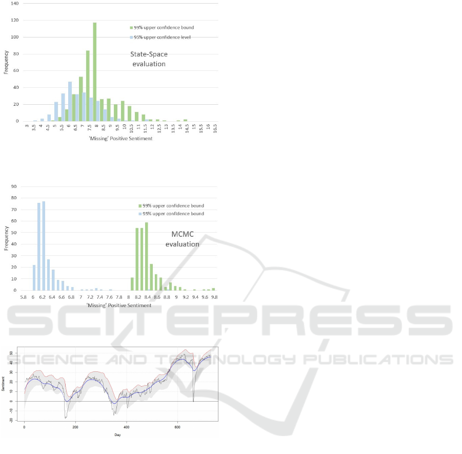
Figure 4: ”Missing positive sentiment” distributions, all or-
ganisations, using the State-Space evaluation (3.7).
Figure 5: ”Missing positive sentiment” distributions, all or-
ganisations, using the MCMC evaluation (3.8).
Figure 6: Amex reputation profile. Black trace: observed
sentiment. Blue trace: smoothed observed. Red dotted
trace: upper 95% confidence bound for the State-Space rep-
resentation. Day range: October 2021 to September 2023
(730 days). The grey region marks the 95% error margin.
The lower confidence bound is not shown but is at the lower
boundary of the grey region.
erature review are that excess negative sentiment does
exist in many contexts. Its origin lies in an innate psy-
chological negative bias. An examination of reputa-
tion time series reveals a very mixed picture. It ap-
pears that factors such as the method of sampling, the
mode of analysis of the samples, and sample location
are all significant factors. Consider, first, the way in
which data are procured and processed. Data feeds
are set up to source texts targeted on particular key-
words. NLP is used to extract sentiment from each,
and an averaging process then determines daily senti-
ment from the texts received during the day. The en-
tire process is automatic and objective, and is geared
to corporate organisations by up-weighting sources
from ’traditional’ media (the press and broadcasting).
Social media, in many cases, is a minor component of
sentiment, except in contentious cases. This method
of data sourcing and analysis differs from the the stud-
ies in the literature review in the following ways.
• The type of sentiment sourced: corporate affairs,
product review, or social comment.
• The calculation method for opinion and senti-
ment.
• The sentiment source.
• The measurement period: one-off or extended.
The second significant determinant of ”missing posi-
tive sentiment” is sampling. The original sample for
this analysis (Section 3.4) was selected on the basis of
industry coverage, which was not a random sample.
The stock index results are derived from predefined
groups, which makes them representative of a partic-
ular class of corporates. It was not possible to draw
a truly random sample from all data available, since
a necessary part of downloading the data is to target
specific organisation names rather than unique identi-
fiers. Therefore, stock index constituents are as near
as we can get to a random sample.
A third factor is also apparent. There appears to
be a regional difference in measuring missing positive
sentiment in the context of reputation. The analysis
of the FTSE and Hang Seng data show precisely the
reverse ’missing’ sentiment compared to data from
other locations. This may indicate a more negative
economic outlook in the UK and Hong Kong/China.
The consequence of these differences is that we might
not expect consistency with previous analyses of neg-
ative bias.
The ”missing positive sentiment” figures in Tables
2 and 3 (Section 4.2) show that at the 95% signifi-
cance level, acceptable consistency is returned by the
State-Space and MCMC methods. Focussing on those
figures, the measured ”missing positive sentiment” is
approximately 6.5 (95% confidence), and 8.4 (99%
confidence), measured on a scale [-100,100]. In per-
centage terms, that scales to 3.25% with respect to
the measured sentiment, independent of scale. Us-
ing the 99% confidence figures, the equivalent fig-
ure is 4.2% of the measured sentiment, independent
of scale. We therefore propose a figure for ”miss-
ing positive sentiment” between 3.25% and 4.2%, and
suggest a ’round’ 4% to account for some long tails
with the MCMC assessment. A simple practical way
in which to apply the 4% figure for ”missing positive
Is Positive Sentiment Missing in Corporate Reputation?
79

sentiment” is to inflate all positive sentiment figures
by 4%, leaving negative sentiment figures unchanged.
The results of this study are significant for two rea-
sons. First, quantification of negative bias using au-
tomated methods coupled with exhaustive data min-
ing is a much more reliable than one-off survey meth-
ods. Therefore, we can place considerable reliance on
the final proposed figure of 4%. Second, the discrep-
ancy between the positive/negative sentiment balance
shows that the context in which measurement takes
place (sources and media), and geographical region
are both important. Generalisation to other contexts
and regions is unsafe.
ACKNOWLEDGEMENTS
We acknowledge the continuing support and assis-
tance of the staff of Penta Group.
REFERENCES
Antypas, D., P. A. and Camacho-Collados, J. (2023). Nega-
tivity spreads faster: A large-scale multilingual twitter
analysis on the role of sentiment in political commu-
nication. In Online Social Networks and Media 33.
doi:10.1016/j.osnem.2023.100242.
Bellovary, A., Y. N. and Goldenberg, A. (2021). Left-
and right-leaning news organizations’ negative tweets
are more likely to be shared. In PsyArXiv 24.
doi:10.31234/osf.io/2er67.
Carter, C. K. and Kohn, R. (1994). On gibbs sampling for
state space models. In Biometrika, 81(3), pp. 541–53.
doi:/10.2307/2337125.
Chomsky, N. (1957). Syntactic structures. Mouton.
Ferrara, E. and Yang, Z. (2015). Quantifying the effect
of sentiment on information diffusion in social media.
In Jnl. Compututer Science 1(51). doi:10.7717/peerj-
cs.26.
Finkelstein, S. R. and Fishbach, A. (2012). Tell me what i
did wrong: Experts seek and respond to negative feed-
back. In Journal of Consumer Research, 39(1), 22–38.
https://doi.org/10.1086/661934.
Fruehwirth-Schnatter, S. (1994). Data augmentation and
dynamic linear models. In Journal of Time Se-
ries Analysis, 15(2), pp. 183–202. doi:10.1111/j.1467-
9892.1994.tb00184.x.
Harvey, A. (1990). Forecasting, structural time series mod-
els and the kalman filter. In Cambridge University
Press.
Hu, N, . P. P. and Zhang, J. (2007). Why do online prod-
uct reviews have a j-shaped distribution? NYU Stern
Business School http://hdl.handle.net/2451/14951.
Liu, B. (2015). Sentiment Analysis: Mining Opinions, Sen-
timents and Emotions. CUP, New York, 1st edition.
Loke, R. and Kisoen, Z. (2022). The role of fake review
detection in managing online corporate reputation. In
Proc, 11th International Conference on Data Science,
Technology and Applications (DATA 2022), pp 245-
256. ScitePress doi:10.5220/0011144600003269.
Loke, R. and Vergeer, J. (2022). Exploring corporate repu-
tation based on sentiment polarities that are related to
opinions in dutch online reviews. In Proc, 11th Inter-
national Conference on Data Science, Technology and
Applications (DATA 2022), pp 423-431. ScitePress
doi:10.5220/0011285500003269.
Mitic, P. (2015). Improved goodness-of-fit tests for opera-
tional risk. In Journal of Operational Risk, 15(1), pp
77-126. Incisive Media doi:10.21314/JOP.2015.159.
Mitic, P. (2017). Standardised reputation measure-
ment. In IDEAL 2017, Guilin China (H. Yin
et al., eds.), LNCS 10585 534-542. Springer:
https://link.springer.com/chapter/10.1007/978-3-319-
68935-7 58.
Moe, W. and Schweidel, D. (2012). Online prod-
uct opinions: Incidence, evaluation and evolu-
tion. In Marketing Science, 31(3) , pp. 372–386.
https://doi.org/10.1287/mksc.1110.0662.
Moe, W. and Schweidel, D. (2013). Positive, negative
or not at all? what drives consumers to post (accu-
rate) product reviews? In Insights 5(2), pp. 8–12.
doi:10.2478/gfkmir-2014-0011.
OpenAI (2019). Better language models and their impli-
cations. https://openai.com/research/better-language-
models.
Park, K., C. M. and Rhim, E. (2018). Positiv-
ity bias in customer satisfaction ratings. In
Proc. WWW ’18, Lyon France, pp. 631-638.
doi.org/10.1145/3184558.3186579.
Powell, D., Y. J. D. M. and Holyoak, K. J. (2017). The
love of large numbers: A popularity bias in consumer
choice. In Psychological Science, 28(10), pp. 1432-
1442. doi.org/10.1177/0956797617711291.
Reichheld, F. F. (2003). The one number you need
to grow. In Harvard Business Review 81(12)
pp. 46–54. https://hbr.org/2003/12/the-one-number-
you-need-to-grow.
Rozin, P. and Royzman, E. B. (2001). Negativity bias,
negativity dominance, and contagion. In Personal-
ity and Social Psychology Review. 5(4) pp. 296–320.
doi:10.1207/S15327957PSPR0504 2.
Shumway, R. and Stoffer, D. (2016). Time Series Analy-
sis and Its Applications With R Examples: Chapter 6.
Springer.
Stieglitz, S. and Dang-Xuan, L. (2013). Emotions
and information diffusion in social media–sentiment
of microblogs and sharing behavior. In Jnl.
Management Info. Systems 29(4) pp. 217–247.
doi:10.2753/MIS0742-1222290408.
Tsugawa, S. and Ohsaki, H. (2017). On the relation be-
tween message sentiment and its virality on social me-
dia. In Social Network Analysis and Mining 7(1):19.
doi:10.1007/s13278-017-0439-0.
Yeo, I.-K. and Johnson, R. A. (2000). A new fam-
ily of power transformations to improve normal-
DATA 2024 - 13th International Conference on Data Science, Technology and Applications
80

ity or symmetry. In Biometrika, 87, pp. 954-959.
doi:10.1093/biomet/87.4.954.
Zendesk (2013). Customer service and Business results: a
survey of customer service from mid-size Companies.
Zendesk.com, http://cdn.zendesk.com/resources/wh
itepapersZendesk\ WP\ Customer\ Service//\ and
\ Business\ Results.pdf, 1st edition.
Is Positive Sentiment Missing in Corporate Reputation?
81