Random Neural Network Ensemble for Very High Dimensional Datasets

Jesus S. Aguilar–Ruiz

1 a

and Matteo Fratini

2 b

Pablo de Olavide University, ES–41013, Spain

Pharmagest, Italy

Keywords:

Neural Network, Ensemble, Random Forest, Very High Dimensionality.

Abstract:

This paper introduces a machine learning method, Neural Network Ensemble (NNE), which combines en-

semble learning principles with neural networks for classiﬁcation tasks, particularly in the context of gene

expression analysis. While the concept of weak learnability equalling strong learnability has been previ-

ously discussed, NNE’s unique features, such as addressing high dimensionality and blending Random Forest

principles with experimental parameters, distinguish it within the ensemble landscape. The study evaluates

NNE’s performance across ﬁve very high dimensional datasets, demonstrating competitive results compared

to benchmark methods. Further analysis of the ensemble conﬁguration, with respect to using variable–size

neural networks units and guiding the selection of input variables would improve the classiﬁcation perfor-

mance of NNE–based architectures.

1 INTRODUCTION

Classifying patient conditions, whether binary or

multiple, through machine learning (ML) algorithms

has long been a focal point in both medicine and

bioinformatics. This paradigm ﬁnds signiﬁcant ap-

plication in the analysis of gene expression proﬁles,

which represent the differential expression of genes in

individuals, often obtained through sequencing tech-

niques such as RNA–Seq. Differences in gene expres-

sion levels typically signify alterations in the cellu-

lar, tissue, or even organismal states. By analyzing

these proﬁles, characteristic patterns for various dis-

eases can be identiﬁed and annotated based on the ob-

served under or over–expression of genes compared

to a reference, which is conventionally established.

Cancer gene expression data is notably complex

due to the prevalence of single nucleotide poly-

morphism (SNP) mutations occurring throughout the

genome. This results in a correspondingly large num-

ber of features (dimensions) to consider, often encom-

passing the most representative genes associated with

the disease. Managing this type of datasets with tens

of thousands of dimensions can encounter the curse

of dimensionality, a concept originally articulated in

(Bellman, 1961), which underscores the challenge of

uncovering latent structures in datasets with a high

https://orcid.org/0000-0002-2666-293X

https://orcid.org/0009-0002-0034-9694

variability of variables. As the number of explanatory

variables increases, so does the complexity of iden-

tifying these structures, particularly evident in tasks

like feature selection for model ﬁtting (Trunk, 1979).

The curse of dimensionality encapsulates the ex-

ponential increase in complexity, especially pro-

nounced in intricate problems with numerous vari-

ables, rendering dimensionality overwhelmingly dif-

ﬁcult to manage (Wellinger and Aguilar-Ruiz, 2022).

Therefore, it becomes imperative to employ tech-

niques for dimensionality reduction, ensuring that in-

formation loss is minimized in the process.

Over the past two decades, ML approaches have

offered a robust framework for resolving gene ex-

pression classiﬁcation problems (Hwang et al., 2002;

Deng et al., 2019). With a diverse range of method-

ologies available, new techniques called Ensembles

have emerged, combining existing methods and of-

ten proving more successful than individual ones (Cai

et al., 2020). This realization has spurred further ex-

perimentation in the ﬁeld. Interestingly, theoretical

work by L. Valiant in the 1980s (Valiant, 1984), con-

ﬁrmed by Schapire in the 1990s (Schapire, 1990),

and subsequently popularized by Surowiecki in 2004

(Surowiecki, 2004), suggests that multiple weak clas-

siﬁers may perform as well as or even better than a

single strong classiﬁer. Building on this idea, Neural

Network Ensembles (NNE) have emerged as a pow-

erful ML model design. NNEs involve ensemble clas-

368

Aguilar–Ruiz, J. and Fratini, M.

Random Neural Network Ensemble for Very High Dimensional Datasets.

DOI: 10.5220/0012763800003756

Paper published under CC license (CC BY-NC-ND 4.0)

In Proceedings of the 13th International Conference on Data Science, Technology and Applications (DATA 2024), pages 368-375

ISBN: 978-989-758-707-8; ISSN: 2184-285X

siﬁers that combine predictions from neural networks

trained on the original dataset, which offers another

promising approach to classiﬁcation problems. How-

ever, when the number of variables is extremely large,

training many networks is prohibitively time consum-

ing. Thus, reducing the size of each of the neural net-

work units that comprise the ensemble could be a vi-

able alternative for an effective classiﬁcation model.

Several ML algorithmic solutions are now avail-

able for gene expression classiﬁcation problems.

However, for the sake of brevity, this work focus on

two main components of the approach presented here:

Neural Networks (NN) (Lancashire et al., 2009) and

Random Forests (RF) (Breiman, 2001). Both NN and

RF have found applications across various ﬁelds over

the years. NNs are represented by a series of layers

of neurons, whose activations depend on an activa-

tion function and connected weights, extending to the

deepest output neurons. Various architectures have

been developed for NN, such as convolutional, feed-

forward, or recurrent NN. However, a drawback is

that the number of hidden neurons and layers need

to be set beforehand, and there is usually no indica-

tion of proper conﬁgurations unless experiments have

been conducted for speciﬁc cases. Random Forests,

on the other hand, are an ensemble learning method

that constructs a multitude of decision trees (Kings-

ford and Salzberg, 2008) during training. They output

the class that is the mode of the classes (classiﬁcation)

or mean prediction (regression) of the individual de-

cision trees.

The aim of this paper is to describe and exper-

imentally demonstrate that NNE can effectively re-

place existing methods in classifying very high di-

mensional biological data. Despite originating from a

theoretical concept proposed in the 1980s, this study

offers a novel focus on addressing the challenge of

very high dimensionality with an ensemble of NNs.

The model will need to address datasets with several

thousands of variables, requiring appropriate NNs ca-

pable of handling millions of parameters. However,

decomposing the problem into pieces, each of which

using lower dimensionality, could reduce the com-

plexity while maintaining the classiﬁcation perfor-

mance. To achieve this goal, the principles of RF will

be employed, where several NNs will be trained and

combined in an ensemble.

Through an exhaustive analysis of the model con-

ﬁguration, this approach also aims to outperform ex-

isting methods in the scientiﬁc literature for predict-

ing real biomedical datasets, particularly gene expres-

sion data on cancer. An experimental analysis of

the predictive power of NNE with ﬁve public cancer

datasets will be shown.

The paper will be organized as follows. Next, re-

lated approaches to the developed method will be de-

scribed. Subsequently, a more in–depth explanation

of the method will be given. Then, after the datasets

employed in the study and the design, with more

stress on the Keras architecture, will be outlined, the

results will be displayed and commented. As a sum-

mary of what has been concretely accomplished with

this study, it is safe to admit that the results achieved

for the proposed method can be reckoned to be gener-

ally positive. This statement can be made considering

the datasets on which it has been tested were classi-

ﬁed on average more poorly by other well–known ML

models.

2 RELATED APPROACHES

The ML approaches described in this paper are in-

trinsic to the method developed and described here.

Through deep learning, these models can extract

higher–level features from raw input data. This ca-

pability provides a powerful approach, particularly in

situations where manual ﬁltering beforehand is chal-

lenging. Deep architectures encompass various vari-

ants of fundamental approaches (Nielsen, 2018). The

diversity within these architectures has led to success

in speciﬁc domains. Deep Neural Networks (DNNs)

have demonstrated high versatility in the ML world.

Signiﬁcant experimentation is dedicated to this archi-

tecture, often coupled with other robust models to im-

prove performance according to the desired solution.

Convolutional Neural Networks (CNNs) are charac-

terized by layers that perform convolutions. Typi-

cally, these layers include multiplication or other dot

product operations, pooling layers, fully connected

layers, and normalization layers. This sophisticated

architecture is particularly effective in tissue image

processing (Browne and Ghidary, 2003). Recurrent

Neural Networks (RNNs) have found applications in

analyzing biological sequences. Furthermore, other

ensembles incorporating neural networks into their

structure have been developed, with some of them

achieving high notoriety (Zhou et al., 2002). In this

work, we will focus on deep fully–connected NN.

RFs are another robust machine learning method,

suitable for both classiﬁcation and regression tasks,

which has gained considerable success over the years

and paved the way for other ensemble learning meth-

ods. RF has consistently proven to be applicable and

reliable in many instances, offering reliability through

a combination of classiﬁers that are varied (high vari-

ance) but predict with very similar accuracy. Ensem-

bles can be developed by varying individual com-

Random Neural Network Ensemble for Very High Dimensional Datasets

369

ponents of the method, such as training data, mod-

els, and combinations. Generally, bagging, boost-

ing, and stacking are the most common techniques for

creating an ensemble (Graczyk et al., 2010). Bag-

ging (Breiman, 1996), as seen in Random Forests,

utilizes bootstrap sampling to obtain subsets of data

for training the base learners. For aggregating the

outputs of these base learners, bagging employs vot-

ing for classiﬁcation tasks and averaging for regres-

sion. Boosting (Freund, 1990), exempliﬁed by Ad-

aboost (Freund and Schapire, 1995), ﬁts a sequence

of weak learners—models whose accuracy is slightly

better than random guessing—to weighted versions of

the data. Examples that were misclassiﬁed by ear-

lier rounds gain more weight. Predictions are then

combined through a weighted majority vote for clas-

siﬁcation or a weighted sum for regression to pro-

duce the ﬁnal prediction. Stacking (Wolpert, 1992)

combines multiple classiﬁcation or regression mod-

els, making it more heterogeneous than other meth-

ods, via a meta-classiﬁer or a meta-regressor, respec-

tively. The base models are trained on a complete

training set, and then the meta-model is trained on the

outputs of the base models as features. While bag-

ging, boosting, and stacking are common techniques,

many other variants exist and can be designed to bet-

ter adapt to speciﬁc problems (Zhou, 2012).

The seminal work on ensemble of neural networks

was focused on providing a number of neural net-

works, all of them dealing with the original input size

(number of variables), in order to reduce the global er-

ror (Hansen and Salamon, 1990). It was demonstrated

that if each network can produce the right prediction

more than half the time, then the likelihood of an er-

ror by a majority decision decreased, and therefore the

ensemble error rate tended to zero when the number

of neural networks tended to inﬁnite. This idea is in-

teresting, but replicating the original input size many

times is very time consuming, and practically unaf-

fordable in cases of very high dimensionality, such as

genomic datasets.

The subject of this study is NNE, a variant of

ensemble techniques that combines DNN architec-

tures with concepts from RF. The choice of using

NN as base classiﬁers in the ensemble was due the

good performance in varied domains. The strategy

employed here follows the principles of RF dataset

splitting criteria, with NN incorporation and param-

eter value selection occurring subsequently using the

same criterion as RF, as described in more detail in the

method section. In terms of computational complex-

ity, training a single large NN on high–dimensional

datasets, as included in this study, would be pro-

hibitively time–consuming due to the large number

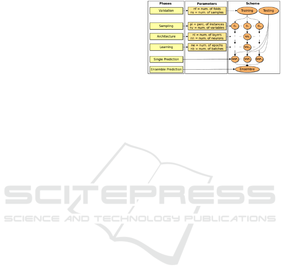
Figure 1: Neural Network Ensemble method representation.

of hyper–parameters involved. In contrast, NNE sig-

niﬁcantly reduces cost by using smaller NNs, which

require less training time. Moreover, increasing the

number of NNs in the ensemble only incurs linear

complexity. The developed method would be advan-

tageous in contexts where other ensemble techniques

are typically applied.

3 METHOD

The principle behind NNE involves training multiple

small NNs on random subsets of the original dataset.

Even a small subset of the entire variable set can pro-

vide valuable information, and each vote in the en-

semble is decisive on its own. This approach helps

reduce bias because each perspective offers a unique

viewpoint. When dealing with very high dimensional

datasets, it is important to verify that small, precise

models can substantially contribute to the overall clas-

siﬁcation performance. This assumption is rooted in

the theory of weak learnability, as proposed by Valiant

(Valiant, 1984), which provides substantial evidence

that strong and weak learnability are equivalent con-

cepts. In essence, it suggests that a model of learnabil-

ity in which the learner needs to perform only slightly

better than random guessing is as effective as a model

in which the learner’s error can be minimized arbi-

trarily. Building upon this assumption, it is reason-

able to hypothesize that an ensemble classiﬁer com-

posed of small weak classiﬁers (such as NNs) could

achieve performance equal to or better than that of a

single larger classiﬁer (a single, huge NN), with sig-

niﬁcantly reduced computational complexity (Shalev-

Shwartz and Singer, 2008).

The method is illustrated in Figure 1 and consists

of six phases, each involving multiple parameter set-

tings. Optimizing each parameter is crucial for max-

imizing the method’s effectiveness, but determining

the best combination within the parameter space can

be challenging. Parameter tuning is computationally

expensive and often requires testing numerous com-

DATA 2024 - 13th International Conference on Data Science, Technology and Applications

370

binations. However, optimizing the parameters of a

set of small NNs is typically less expensive than opti-

mizing a single, large NN.

Let M represent the number of variables and N

represent the number of instances in the dataset. The

parameters deﬁning the overall structure of the model

are listed in order of implementation by the method:

• n f : number of folds.

• ns: number of samples.

• nv: number of variables at each sample.

• pi: percentage of instances.

• nl: number of layers.

• nn: number of nodes.

• ne: number of epochs.

• nb: number of batches.

The parameters n f and ns are set at the beginning for

validation. n f can be chosen according to the needs

and goals of the experiment, whereas ns requires an

automatic adjustment based on dataset dimensional-

ity evaluation. More speciﬁcally, the adjustment is

performed by means of a mathematical expression re-

lated to nv. Considering that ns would depend on

the probability of not choosing a single variable after

ns extractions with replacement, in order to guaran-

tee that the probability P of not using any variable in

the model would be minimal after ns extractions of nv

variables, the following Eq. 1, that shows the relation

between P and nv, ns and M need to be analyzed.

P =

1 −



M−1

nv−1







(1)

Eq. 1 can be simpliﬁed in order to relate the prob-

ability with the number of samples and the number

of variables at each sample, thus neglecting the bino-

mial coefﬁcients, as shown in Eq. 2. As the number

of selected variables and the number of samples in-

crease, the probability tends to zero. Indeed, we found

a reasonable compromise by setting the value for P as

P =

√

(for instance, for a dataset with 30,000 genes,

P ≈ 0.005). This value represents a very low proba-

bility when the number of variables M is large, as is

often the case with genomic data.

P =



1 −



(2)

The parameter nv is deﬁned for the sampling pha-

se, where dimensionality reduction occurs. Although

set at the beginning along with ns, it is important

to note that the splitting is executed after specifying

the value of ns. The value of nv is established by

the expression found as the splitting criterion in RF,

i.e., nv =

√

M, which has already proven to be effec-

tive with decision trees. Thus, the number of samples

could be calculated as shown in Eq. 3.

ns =

log

√

log



1 −

√



(3)

For example, the Prostate GSE6919 U95B dataset,

with 12,621 variables, would require 526 samples of

112 variables to satisfy the condition. Similarly, the

Bladder GSE31189 dataset, with 54,676 variables,

would need 1,274 samples of 234 variables.

The parameter pi plays an important role when

the number of instances in the dataset is high, such

that reducing this dimension contributes to improve

the computational cost. However, in genomic datasets

it is not common to ﬁnd a large number of instances,

unlike in clinical datasets. Therefore, the parameter

pi was set to 100% for all the experimental analysis,

as the number of instances ranges from 20 to 124.

During the architecture phase, Keras was em-

ployed for designing the architecture and deﬁning pa-

rameter values (nl, nn). The architecture was inten-

tionally kept simple by ﬁxing the nl parameter at a

value of 2, indicating two dense layers plus an output

layer. The value of nn was derived from an expres-

sion that uses the number of input neurons calculated

in nv, as shown in Eq. 4.

nn =



√

log

√



(4)

The parameters nb and ne were speciﬁed for the

learning phase, which is common in deep learning

where multiple passes over the same training set may

be necessary to enhance the overall predictive power

of the model. In this case, ne was limited to 500. This

decision was based on ensuring a sufﬁcient number of

passes over the training dataset. Although the upper

bound of 500 epochs was chosen, it was rarely nec-

essary to reach that limit due to the inclusion of an

early stopping criterion. Speciﬁcally, the minimum

delta was set to 0.005 over the training loss, with a

patience of 20 epochs (i.e., if after 20 epochs the per-

formance does not improve, then the learning stops).

With this condition, the majority of training processes

(over 95%) required between 85 and 95 epochs. The

value of nb was established to be about one sixth of

the averaged number of instances (i.e., 15).

Once a classiﬁer was trained according to the pre-

viously explained scheme, it predicted on new ex-

amples and the respective assignments were stored.

Due to the intrinsic randomness in the method, the

same examples would likely be predicted by multiple

classiﬁers. Subsequently, when all predicted labels

Random Neural Network Ensemble for Very High Dimensional Datasets

371

for each example were collected, the class mode was

computed. Thus, the most frequent vote per example

was selected as the class with the highest probability

among all classiﬁers’ votes.

The advantages of the NNE over any deep fully–

connected NN is notorious regarding the ability of

learning in local subspaces, which is much less ex-

pensive.

4 EXPERIMENTAL ANALYSIS

4.1 Datasets

The study includes ﬁve datasets on gene expression

proﬁles data from various types of cancers in hu-

man patients. In these datasets, genes represent the

variables, with cells containing the expression values,

while samples represent observations of sets of vari-

ables. The raw data underlying the datasets was ob-

tained using microarray technology and deposited in

the Gene Expression Omnibus (GEO) repository by

other authors. Prior to the processing phase described

in this paper, the collected datasets underwent prepro-

cessing by manual curation. This preprocessing in-

volved considerations such as sample quality assess-

ment, removal of unwanted probes, background cor-

rection, and normalization. All relevant information

regarding to the datasets is summarized in Tab. 1,

where names denote the anatomical section where the

cancer is localized, with appended codes representing

their indexing in the GEO database. For further de-

tails about the datasets, interested readers can refer to

the Structural Bioinformatics and Computational Bi-

ology Lab (SBCB Lab) website (Feltes et al., 2019).

The Colorectal GSE44861 dataset presents 105

samples, 22,278 genes and 2 classes,53 normal and 47

tumoral state classes. The Breast GSE59246 dataset

has 101 samples, 36,623 genes and 2 classes iden-

tifying a DCIS (Ductal Carcinoma In Situ) and a

IBC (Invasive Breast Cancer) respectively, two types

of cancer interesting the breast section. 45 patients

were diagnosed with DCIS and 56 with IBC. The

Bladder GSE31189 dataset has 85 samples, 54,676

genes, a tumoral urothelial and a normal urothelial

class. 34 normal against 51 tumoral patients could be

collected overall, showing the dataset certain imbal-

ance. The Renal GSE53757 dataset has only 20 sam-

ples, 22,284 genes and CCRCC (clear cell renal cell

carcinoma) class along with the normal state class.

It represents the most balanced dataset with 10 pa-

tients in normal and tumoral states, respectively. The

Prostate GSE6919 U95B dataset includes 124 sam-

ples, 12,621 genes and primary prostate tumor class

representing the disease condition and a normal state

class. Higher class balance can be achieved in this

case, with 60 patients in normal conditions and 64

suffering from prostate cancer. In general, it is quite

difﬁcult to learn in high–dimensional spaces from so

few instances without overﬁtting. The diversity pro-

vided by the NNE model helps to mitigate this issue.

4.2 Design

The method integrated a NN architecture as training

components (base classiﬁers) and compared them to

accelerate computational time while improving good

performance. In order to make fair comparisons be-

tween NNE and a single NN, many parameters were

set the same manner. However, the NNE architec-

ture, as described in previous section, is composed of

a number of very simple NN units, instead of a unique

large NN architecture.

Multi–Layer Perceptron (MLP), being the most

basic type of NN, is a reliable ML model for vari-

ous classiﬁcation problems due to its extensive use in

research projects and benchmarks. In MLP training,

the RMSProp (Root Mean Square Propagation) algo-

rithm –a variant of the RProp (Resilient Propagation)

algorithm (Riedmiller and Braun, 1993)– is employed

to decrease training time.

The Keras architecture for MLP comprises two

dense layers, each with the number of nodes obtained

by Eq. 4, and employs Rectiﬁed Linear Units (ReLU)

as the activation function for the ﬁrst two layers and

softmax for the output layer. ReLU activation func-

tions are commonly used in neural networks due to

their ability to speed up training by simplifying gradi-

ent computation. The softmax function, chosen for

the last layer, converts a real vector into a vector

of categorical probabilities, enabling interpretation of

results as a probability distribution.

To improve generalization, speciﬁc regularizers

were incorporated to both MLP and NNE to apply

penalties on layer parameters and activity during opti-

mization. An Elastic Net regularization, which com-

bines the features of both L1 and L2 regularization,

was selected. This regularization eliminates the limi-

tations found in L1 regularization by estimating both

the median and mean of the data to avoid overﬁtting.

It is considered more appropriate when the dimen-

sional data exceeds the number of samples used, mak-

ing it well–suited for the case of genomic datasets,

with few samples and many variables present.

Additionally, the Glorot normal method was cho-

sen as the initializer. NNs are known to be sensitive

to initial weight values, necessitating consideration of

more complex initializers for achieving better results.

DATA 2024 - 13th International Conference on Data Science, Technology and Applications

372

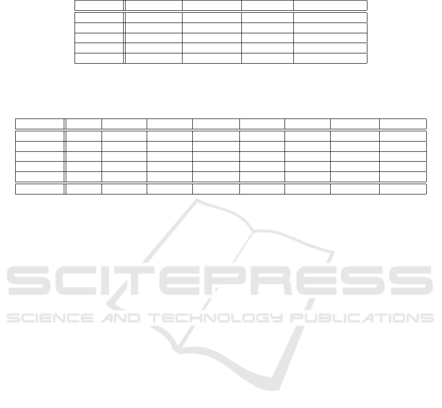
Table 1: Description of the ﬁve gene expression proﬁle datasets on human cancer. The datasets were selected from the SBCB

Lab archive. The name, number of genes, instances, classes, and class distribution of each dataset are in columns.

Dataset No. of genes No. instances No. classes Class distribution

Colorectal 22278 105 2 53:47

Breast 36623 101 2 45:56

Bladder 54676 85 2 34:51

Renal 22884 20 2 10:10

Prostate 12621 124 2 60:64

Table 2: Description of the Neural Network–based architectures, both MLP and NNE. Var: number of variables; MLP inp:

number of input neurons for MLP; MLP hid: number of neurons in the hidden layers; MLP par: total number of parameters

for MLP; NNE inp: number of input neurons for each simple NN; NNE hid: number of neurons in the hidden layer for NNE;

NNE units: number of simple NN for the NNE; NNE par: total number of parameter for the NNE architecture.

Dataset Var. MLP inp. MLP hid. MLP par. NNE inp. NNE hid. NNE units NNE par.

Colorectal 22,278 22,278 69 1,539,127 149 11 743 110,719

Breast 36,623 36,623 84 3,085,651 191 12 1001 191,.106

Bladder 54,676 54,676 99 5,416,637 234 13 1274 298,073

Renal 22,884 22,884 55 697,579 112 10 526 58,924

Prostate 12,621 12,621 69 1,597,909 151 11 755 114,020

Mean 31,550 31,550 77 2,684,749 172 12 886 2,025,484

No constraints were speciﬁed in any layer, allowing

ﬂexibility in model optimization.

To prevent overﬁtting in the MLP, the early stop-

ping technique was implemented as a form of regular-

ization, with a patience of 20 epochs (the number of

epochs with no improvement after which training will

be stopped) and a minimum delta of 0.005 (the min-

imum change in the monitored quantity to qualify as

an improvement). These values were chosen to make

fair comparisons to the NNE approach.

Given the number of input neurons for the MLP,

which incorporates quite complexity in the learning

phase, the number of epochs was set to 5,000, al-

lowing more potential room for improvement, and the

batch size was set to 15, with the training data shufﬂed

before each epoch.

The training sets underwent min–max normaliza-

tion, scaling the values between 0 and 1. The normal-

ization parameters obtained from the training set were

then used to normalize the test set in the same manner.

For all experiments, 3–fold cross–validation was

employed for validation, with stratiﬁed sampling used

to ensure homogeneous splitting of the classes at ev-

ery iteration. This number of folds was chosen to al-

low a fair comparison with the results published in

(Feltes et al., 2019) using the same datasets with other

classiﬁers. In order to compare the size of both ar-

chitectures, in terms of difﬁculty of parameter opti-

mization, Tab. 2 describes the complexity of both

MLP and NNE. The NNE architecture compared to

the MLP needs, on average, less amount of parame-

ters to be optimized.

Benchmarking was conducted by considering sev-

eral ML models, including Na

ıve–Bayes, Random

Forest, k–Nearest Neighbors, and MLP. These models

had previously been run by other authors on the ﬁve

selected datasets, with dimensionality reduction tech-

niques such as t–SNE and PCA applied to the original

data. Evaluation of results was based on accuracy and

the area under the ROC curve as metrics.

Technically, the approach was developed on the

KNIME (Berthold et al., 2007) data analytics plat-

form, which offers a variety of functional nodes for

machine learning. Additionally, the integration of the

Keras (Chollet et al., 2015) library for deep learning

provided the necessary tools for implementing NNs

within the KNIME framework.

4.3 Results

To ease replicability, several well–known classiﬁers

have been chosen: Na

ıve–Bayes (NB), Multi–Layer

Perceptron (MLP,) Random Forests (RF) and k–

Nearest Neighbors (kNN). All these ML algorithms

are commonly employed in microarray gene expres-

sion analysis, and generally present a good overall

performance. Upon running NNE on the ﬁve speci-

ﬁed datasets with a 3–fold cross–validation, the fol-

lowing ﬁndings emerged.

For the Bladder dataset, an overall accuracy of

0.553 was recorded. The area under the ROC curve

was computed at 0.601. Notably, the accuracy for

Bladder was comparable to RF and lower than any

other considered algorithm, apart from NB, even

though the average performance did not exceed 0.64.

For to the Prostate dataset, similarly low values

were observed. The accuracy calculation yielded a

value of 0.67, in line with other methods. However,

Random Neural Network Ensemble for Very High Dimensional Datasets

373

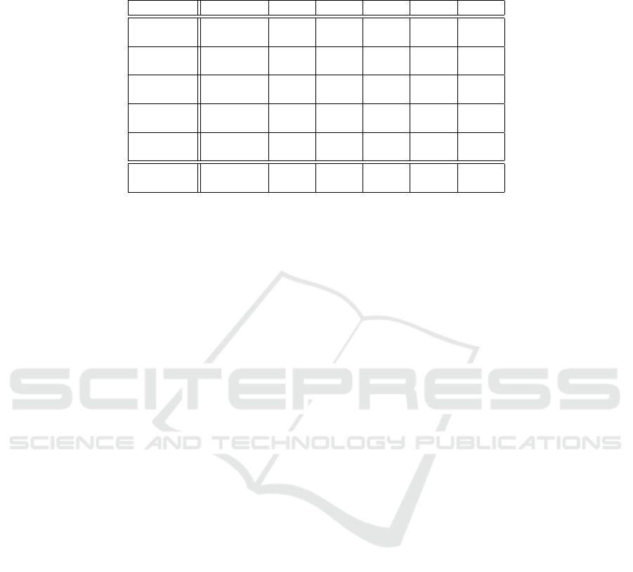
Table 3: Classiﬁcation performance comparative analysis. Acc: classiﬁcation accuracy; AU(ROC): area under the ROC

curve; Mean: Last row containing the Acc and AU(ROC) mean for each model over all the datasets; NNE: Neural Network

Ensemble; MLP: Multilayer Perceptron; NB: Na

ıve–Bayes; RF: Random Forests; kNN: k–Nearest Neighbors.

Dataset Measure NNE MLP NB RF kNN

Colorectal

Acc

AU(ROC)

0.87

0.90

0.64

0.72

0.84

0.82

0.87

0.69

0.68

Breast

Acc

AU(ROC)

0.86

0.89

0.60

0.64

0.72

0.70

0.79

0.85

0.73

0.74

Bladder

Acc

AU(ROC)

0.55

0.60

0.58

0.50

0.46

0.55

0.53

0.62

0.63

Renal

Acc

AU(ROC)

0.85

0.80

0.86

0.90

0.85

0.89

0.85

0.80

Prostate

Acc

AU(ROC)

0.67

0.74

0.62

0.63

0.69

0.70

0.67

0.76

0.56

0.59

Mean

Acc

AU(ROC)

0.76

0.80

0.65

0.67

0.72

0.74

0.78

0.69

the area under the ROC curve reported a relatively

good value of 0.743.

In contrast, the Breast dataset displayed consider-

able improvement in metric magnitude average. Ac-

curacy was notably high at 0.861, and an area under

the ROC curve of 0.894, indicating its reliability as

a predictor. Other methods performed inferiorly to

NNE on this dataset, with accuracies below 0.8.

Likewise, the Colorectal dataset yielded results

similar to those of the Breast dataset. Accuracy was

0.867 and area under the ROC curve was 0.901. Other

methods failed to surpass NNE performance on this

dataset, remaining equal or below 0.84.

Training on the Renal dataset, despite its smaller

number of observations, led to satisfactory results.

Accuracy was recorded at 0.85, with the area under

the ROC curve reaching 0.85. Although NB outper-

formed NNE with accuracy values of 0.9, the rest re-

mained close to NNE results.

In comparison with the other algorithms selected

for benchmarking, the proposed method showed an

overall higher performance. In general, according to

related scientiﬁc literature, the choice of the classi-

ﬁcation method for such large number of genes and

small number of cases substantially inﬂuence classi-

ﬁcation success (Pirooznia et al., 2008). That means

that considering the dimensionality reduction carried

out automatically by NNE for each individual model,

the quality of these very small models, and the combi-

nation strategy, the NNE approach is suitable for very

high–dimensional contexts.

5 CONCLUSIONS

A machine learning method has been introduced for

solving classiﬁcation problems, which combines the

principles of ensemble learners and neural networks

with the sampling policy of random forests. While the

concept of weak learnability equalling strong learn-

ability has been discussed extensively in the past,

placing this method in historical context, the main

features of NNE still distinguish it within the ensem-

ble landscape. Speciﬁcally, NNE addresses speciﬁc

challenges related to very high dimensionality (curse

of dimensionality) and model aggregation (overﬁt-

ting).

Although it is known that a single neural network

could address the problem, the very high number of

genes would result in a huge input layer, which would

make the optimization of the underlying parameters

of the architecture complex. In this work, instead, we

show that using many very small NNs, with only two

hidden layers containing few neurons, greatly reduces

the task of learning the weights, while maintaining the

quality of the classiﬁer model.

The results obtained demonstrate that NNE can ef-

fectively classify data across the ﬁve datasets, consis-

tent with other benchmark methods (MLP, SVM, NB,

RF, and kNN). This suggests that NNE could poten-

tially replace other existing methods for classiﬁcation

in the context of very high dimensional gene expres-

sion datasets. In addition, the NNE compared to the

MLP needs, on average, less amount of parameters to

be optimized.

An interesting aspect of the NNE model is that

there is scope for potential improvement. An analy-

sis of the ensemble conﬁguration could provide even

better results by addressing two aspects: a) selecting

a variable number of input neurons for each single

NN; b) using a heuristic (rather than random) to se-

lect which input variables the NNs will use, so that

not all variables are chosen with approximately the

same probability.

DATA 2024 - 13th International Conference on Data Science, Technology and Applications

374

ACKNOWLEDGEMENTS

This work was supported by MCIN/AEI/10.13039/

501100011033 under Grant PID2020-117759GB-I00.

REFERENCES

Bellman, R. (1961). Adaptive Control Processes: A Guided

Tour. Princeton University Press.

Berthold, M. R., Cebron, N., Dill, F., Gabriel, T. R.,

otter, T., Meinl, T., Ohl, P., Sieb, C., Thiel, K.,

and Wiswedel, B. (2007). KNIME: The Konstanz In-

formation Miner. In Studies in Classiﬁcation, Data

Analysis, and Knowledge Organization (GfKL 2007).

Springer.

Breiman, L. (1996). Bagging predictors. Machine Learn-

ing, 24(2):123 – 140. Cited by: 1993; All Open Ac-

cess, Bronze Open Access.

Breiman, L. (2001). Random forests. Machine Learning,

45(1):5 – 32.

Browne, M. and Ghidary, S. S. (2003). Convolutional neu-

ral networks for image processing: An application in

robot vision. In Gedeon, T. T. D. and Fung, L. C. C.,

editors, AI 2003: Advances in Artiﬁcial Intelligence,

pages 641–652, Berlin, Heidelberg. Springer Berlin

Heidelberg.

Cai, Y., Zhang, W., Zhang, R., Cui, X., and Fang, J. (2020).

Combined use of three machine learning modeling

methods to develop a ten-gene signature for the di-

agnosis of ventilator-associated pneumonia. Medical

Science Monitor, 26.

Chollet, F. et al. (2015). Keras.

Deng, J.-L., Xu, Y.-h., and Wang, G. (2019). Identiﬁcation

of potential crucial genes and key pathways in breast

cancer using bioinformatic analysis. Frontiers in Ge-

netics, 10:695.

Feltes, B. C., Chandelier, E. B., Grisci, B. I., and Dorn,

M. (2019). Cumida: An extensively curated microar-

ray database for benchmarking and testing of ma-

chine learning approaches in cancer research. Jour-

nal of Computational Biology, 26(4):376–386. PMID:

30789283.

Freund, Y. (1990). Boosting a weak learning algorithm by

majority. page 202 – 216.

Freund, Y. and Schapire, R. E. (1995). A desicion-theoretic

generalization of on-line learning and an application

to boosting. In Vit

anyi, P., editor, Computational

Learning Theory, pages 23–37, Berlin, Heidelberg.

Springer Berlin Heidelberg.

Graczyk, M., Lasota, T., Trawi

nski, B., and Trawi

nski, K.

(2010). Comparison of bagging, boosting and stack-

ing ensembles applied to real estate appraisal. In

Nguyen, N. T., Le, M. T., and

Swiatek, J., editors,

Intelligent Information and Database Systems, pages

340–350, Berlin, Heidelberg. Springer Berlin Heidel-

berg.

Hansen, L. and Salamon, P. (1990). Neural network en-

sembles. IEEE Transactions on Pattern Analysis and

Machine Intelligence, 12(10):993–1001.

Hwang, K.-B., Cho, D.-Y., Park, S.-W., Kim, S.-D., and

Zhang, B.-T. (2002). Applying Machine Learning

Techniques to Analysis of Gene Expression Data:

Cancer Diagnosis, pages 167–182. Springer US,

Boston, MA.

Kingsford, C. and Salzberg, S. (2008). What are decision

trees? Biotechnology, 26(9):1011–1012.

Lancashire, L. J., Lemetre, C., and Ball, G. R. (2009). An

introduction to artiﬁcial neural networks in bioinfor-

matics—application to complex microarray and mass

spectrometry datasets in cancer studies. Brieﬁngs in

Bioinformatics, 10(3):315–329.

Nielsen, M. A. (2018). Neural networks and deep learning.

Pirooznia, M., Yang, J., Yang, M., and Deng, Y. (2008). A

comparative study of different machine learning meth-

ods on microarray gene expression data. BMC ge-

nomics, 9 Suppl 1:S13.

Riedmiller, M. and Braun, H. (1993). A direct adaptive

method for faster backpropagation learning: the rprop

algorithm. In IEEE International Conference on Neu-

ral Networks, pages 586–591 vol.1.

Schapire, R. (1990). The strength of weak learnability. Ma-

chine Learning, 5(2):197–227.

Shalev-Shwartz, S. and Singer, Y. (2008). On the equiv-

alence of weak learnability and linear separability:

New relaxations and efﬁcient boosting algorithms.

volume 80, pages 311–322.

Surowiecki, J. (2004). The Wisdom of Crowds: Why the

Many Are Smarter Than the Few and How Collective

Wisdom Shapes Business, Economies, Societies and

Nations. Little, Brown and Company.

Trunk, G. V. (1979). A problem of dimensionality: A sim-

ple example. IEEE Transactions on Pattern Analysis

and Machine Intelligence, PAMI-1(3):306–307.

Valiant, L. G. (1984). A theory of the learnable. Commun.

ACM, 27(11):1134–1142.

Wellinger, R. E. and Aguilar-Ruiz, J. S. (2022). A new chal-

lenge for data analytics: transposons. BioData Min-

ing, 15(1):9.

Wolpert, D. H. (1992). Stacked generalization. Neural Net-

works, 5(2):241–259.

Zhou, Z. (2012). Ensemble Methods: Foundations and

Algorithms. CHAPMAN & HALL/CRC MACHINE

LEA. Taylor & Francis.

Zhou, Z.-H., Wu, J., and Tang, W. (2002). Ensembling neu-

ral networks: Many could be better than all. Artiﬁcial

Intelligence, 137(1):239 – 263.

Random Neural Network Ensemble for Very High Dimensional Datasets

375