Artificial Bee Colony Algorithm: Bottom-Up Variants for the Job-Shop
Scheduling Problem
K. A. Yousseffi
a
, M. Gojkovic and M. Schranz
b
Lakeside Labs GmbH, Klagenfurt, Austria
fi
Keywords:
Swarm Intelligence, Bio-Inspired Algorithm, Bee Algorithm, Job-Shop Scheduling, Agent-Based Modeling.
Abstract:
The optimization of a job-shop scheduling problem, e.g., in the semiconductor industry, is an NP-hard prob-
lem. Various research work have shown us that agent-based modeling of such a production plant allows to
efficiently plan tasks, maximize productivity (utilization and tardiness) and thus, minimize production delays.
The optimization from the bottom-up especially overcomes computational barriers associated with traditional,
typically centrally calculated optimization methods. Specifically, we consider a dynamic semiconductor pro-
duction plant where we model machines and products as agents and propose two variants of the artificial
bee colony algorithm for scheduling from the bottom-up. Variant (1) prioritizes decentralization and batch
processing to boost production speed, while Variant (2) aims to predict production times to minimize queue
delays. Both algorithmic variants are evaluated in the framework SwarmFabSim, designed in NetLogo, fo-
cusing on the job-shop scheduling problem in the semiconductor industry. With the evaluation we analyze the
effectiveness of the bottom-up algorithms, which rely on low-effort local calculations.
1 INTRODUCTION
The increased complexity in scheduling of produc-
tion plants organized by the flexible job-shop princi-
ple comes from the dynamics of customized, flexible,
on-demand production that is combined with a high
product diversity. Exemplary for such a production
facility, we consider the semiconductor manufacturer
Infineon Technologies Austria AG
1
. They deal with
comparatively low-volume integrated circuit produc-
tion in the logic and power sector, compared to the
high volumes of memory and CPU manufacturers.
For getting a better idea, exemplary, they produce
1500 products in around 300 processing steps by us-
ing up to 1200 different machines (Schranz et al.,
2021b; Khatmi et al., 2019). All these characteris-
tics lead to an NP-hard problem that does not allow
traditional, linear optimization methods or centrally
pre-computed swarm algorithms (Gao et al., 2019) to
calculate a global optimization of the plant in a rea-
sonable amount of computational time (Lawler et al.,
1993). As proposed in Schranz et al. (Schranz et al.,
2021b), we use the innovative approach to perform
a
https://orcid.org/0000-0002-8719-7699
b
https://orcid.org/0000-0002-0714-6569
1
Infineon Technologies, https://www.infineon.com/
agent-based modelling of the production plant. This
leads to a self-organizing system of agents where each
agent executes local rules, makes decisions based on
local knowledge and locally interacts with agents in
its neighborhood. This modelling approach shifts
the problem of a global computed overall solution
to small, local decisions that lead to a distributed,
self-organized algorithm. Such an optimization from
the bottom-up dynamically reacts on changing envi-
ronmental conditions (e.g., tool downs, processing
loops, product priorities) and produces near-optimal
solutions for the NP-hard job-shop problem. Sev-
eral swarm algorithms already inspired the success-
ful engineering of this bottom-up strategy, including
ants and hormones (Umlauft et al., 2022), or bats and
glowworms (Umlauft et al., 2023a).
In this paper, honeybees serve as inspiration to
derive two variants of swarm intelligence algorithms
from their behavior. Honeybees live in a hive to-
gether, where their main task is to search for pollen
and transport it back to their colony. To increase the
efficiency of food transport, bees attract other bees
by performing a waggle dance. The dance perfor-
mance shows the direction, distance and quality of
the food source. This behavior was originally ab-
stracted and designed as the artificial bee colony algo-
rithm (ABC) (Karaboga and Basturk, 2007). In this
Yousseffi, K., Gojkovic, M. and Schranz, M.
Artificial Bee Colony Algorithm: Bottom-Up Variants for the Job-Shop Scheduling Problem.
DOI: 10.5220/0012765900003758
Paper published under CC license (CC BY-NC-ND 4.0)
In Proceedings of the 14th International Conference on Simulation and Modeling Methodologies, Technologies and Applications (SIMULTECH 2024), pages 103-111
ISBN: 978-989-758-708-5; ISSN: 2184-2841
Proceedings Copyright © 2024 by SCITEPRESS – Science and Technology Publications, Lda.
103

paper we perform the modeling and engineering of
the ABC onto the problem of the semiconductor job-
shop scheduling problem. Therefore, the local rules
are adapted and aligned with the requirements from
the semiconductor production plant model for its op-
timization from the bottom-up. In variant (1), origi-
nally also presented in Umlauft et al. (Umlauft et al.,
2023b), the focus is to keep the algorithm decentral-
ized and put a high priority on feeding batch process-
ing machines to accelerate production. In variant (2),
the goal is to predict the process time for each produc-
tion and avoid long queueing periods. Though these
algorithms are completely different, Variant (2) is de-
veloped by considering the drawbacks of Variant (1).
The paper is organized as follows: In Section 2 we
provide a model of the considered production plant
and give an overview of the relevant related work.
Section 3 describes the natural, but already abstracted
bee behavior and explains the two variants of the en-
gineered ABC algorithms. The corresponding results,
where we compare the two variants against each other
and a so-called baseline algorithm, are described in
Section 4. We conclude the paper in Section 5 and
provide an outlook on future work and possibilities
for further swarm engineering in this domain.
2 BACKGROUND
The typical method to address job-shop scheduling
is linear optimization. Up to now, no solution was
developed that allows an optimization in polynomial
time (Zhang et al., 2009), and thus only consider the
optimization of a subset of a production plant (Lawler
et al., 1993). Therefore, one approach is to agent-
based modeling to engineer the production plant as
a swarm of self-organized agents (Umlauft et al.,
2023b; Schranz et al., 2021b; Umlauft et al., 2022).
As observed in the natural swarm behavior of fish,
ants or birds, the agents use local rules and interac-
tions in their neighborhood to reach a global goal like,
e.g., foraging (Schranz et al., 2021a). Using this ap-
proach, the result leads to an optimization of the pro-
duction plant from the bottom-up instead of calculat-
ing a global optimization solution from the top-down.
2.1 Production Plant Model
The production plant in the considered semiconduc-
tor industry is modeled with a number of products,
so-called lots L
t
= {l
t
1
, l
t
2
, . . . }. Each lot relates to a
specific recipe R
t
to produce a lot of a certain prod-
uct type t. In the recipe we have a prescription on
the process step P
m
i
that must be performed next.
Thus, the recipe is an ordered list of process steps
R
t
= {P
1
, P
2
, . . . }. The production plant runs a num-
ber of machines M, where each machine M
m
i
is of a
machine type m and has a queue Q
m
i
. We differenti-
ate between two kind of machines that again increases
optimization complexity: single-step machines (pro-
cess one lot after the other), and batch-oriented ma-
chines (process a batch of several lots of the same type
t at once). Machines that have the same type m are
grouped into workcenters W
m
⊂ M. Further on, for
every machine or process type m to be performed, at
least one workcenter W
m
containing at least one ma-
chine M
m
of type m must exist. In typical production
plants there exists multiple machines per workcenter
and for each necessary process step P
m
∈ R
t
a lot l
t
n
must decide which of the suitable machines M
m
i
∈ W
m
to enqueue. Depending on the used algorithm, ma-
chines can also re-order their queues Q
m
i
.
2.2 Related Work
The artificial bee colony (ABC) algorithm was al-
ready considered multiple times for the job-shop
scheduling problem (JSSP) as a centrally calculated
algorithm: In (Yao et al., 2010; Han et al., 2012) the
authors proposed the improved ABC (IABC) where
they enhanced the convergence rate. Other works
like in (Gupta and Sharma, 2012) were able to in-
crease the efficiency by implementing additional mu-
tation and crossover operations in the classical ABC
algorithm. Another ABC variant is shown in (Ku-
mar et al., 2014), where the Crossover-based ABC
(CbABC) strengthens the exploitation phase of ABC
as crossover enhances the exploration of the search
space. In (Alvarado-Iniesta et al., 2013) they op-
timized the raw material supply process for differ-
ent production lines in a local manufacturing plant.
In (Yurtkuran and Emel, 2014) they proposed the
modified artificial bee colony (M-ABC) algorithm
with random key-based encoding for solution repre-
sentation and a new multi-search strategy. Another
modified ABC, named Beer froth ABC (Sharma et al.,
2018), solves the JSSP by successfully keeping the
exploration-exploitation balance. Fuzzy processing
time for the FJSP was investigated in (Gao et al.,
2016). For further details on literature the reader is re-
ferred to (Karaboga et al., 2014; Khader et al., 2013).
SIMULTECH 2024 - 14th International Conference on Simulation and Modeling Methodologies, Technologies and Applications
104

3 THE ARTIFICIAL BEE
COLONY ALGORITHM
3.1 The Natural Inspiration
The intelligent behavior of honeybee colonies in-
spired Karaboga (Karaboga and Basturk, 2007) to de-
fine meta-heuristics for solving numerical optimiza-
tion problems. The Artificial Bee Colony (ABC)
algorithm exhibits swarm-based behavior with three
main components: employed and unemployed bees,
and food sources (solutions to a given problem).
Bee agents implement recruitment and abandonment
strategies. This behavior results in positive and neg-
ative feedback necessary for a self-organizing system
and collective intelligence. The Algorithm 1 presents
the pseudo-code of the ABC algorithm. During the
Initialization Phase, algorithmic parameters are ini-
tialized alongside the food source population. Bees in
the Employed Bees Phase are allocated to individual
food sources so that each food source employs only
one bee. In the Onlooker Bees Phase, bees opt for one
of the food sources advertised by the employed bees.
In contrast, scout bees adopt a stochastic selection ap-
proach when discovering a food source. In the Scout
Bees Phase, additionally, an employed bee can transit
to a scout bee when the quality of the advertised food
source is decreased due to excessive exploitation by
onlooker bees or the food source is of inherently low
quality. A more detailed description of the algorithm
and its phases is given in (Umlauft et al., 2023b).
Algorithm 1: ABC as global optimizer.
1: Initialization Phase (population of the food
source)
2: repeat
3: Employed Bees Phase
4: Onlooker Bees Phase
5: Scout Bees Phase
6: Memorize the best solution
7: until Cycle = Maximum Cycle Number or a Max-
imum CPU time
In the vast literature on the ABC algorithm ap-
plied to the JSSP (see Section 2.2), the population of
bees always represent a solution space, i.e., the al-
gorithm is calculated centrally. Our contribution con-
sists of opting for the bottom-up approach, where bees
represent agents (instead of solutions) that follow lo-
cal rules from which a global behavior (the optimal
schedule) emerges. Thus, we present a completely
new approach to the ABC algorithm application.
3.2 The ABC - Variant (1)
The first variant of the ABC algorithm implements
the following mapping to address the JSSP (Umlauft
et al., 2023b):
• food source = machine, M
m
i
∈ W
m
, i = 1, 2, . . . , I
• bee = lot from one product, l
t
n
∈ L
t
, n = 1, 2, . . . , N.
The algorithm is implemented so that each lot l
t
n
follows a recipe R
t
that defines process steps P
m
nec-
essary for lots of type t to complete their production.
Machines of the same type m perform the process P
m
and are grouped in a workcenter W
m
. Since in a lot’s
recipe only a process step P
m
is defined, but not the
specific M
m
i
∈ W
m
, a lot needs to make a decision.
A lot is modeled as an onlooker bee l
OB
or a scout
bee l
SB
. The latter chooses a random machine and
the former will probabilistically choose the best M
m
i
∈
W
m
(Eq. 2). The former selects a random machine
M
m
i
from a workcenter and upon finishing the process,
evaluates the machine’s quality Q(M
m
i
) (Eq. 1) with
Q(M
m
i
) =
1
w
SB
(1)
where w
SB
is the total waiting time of lot l
SB
, i.e., the
time a lot spent waiting in the queue and the process-
ing time of the machine M
m
i
.
P
r
(M
m
i
) =
fit(M
m
i
)
∑
I
i=1
fit(M
m
i
)
(2)
The probability P
r
(M
m
i
), as defined in Eq. 2, is in-
fluenced by the machine’s own fitness fit(M
m
i
) relative
to the sum of fitness values of all machines within
the same workcenter W
m
. Once l
SB
evaluates the ma-
chine’s quality Q(M
m
i
), other incoming l
OB
will have
enough information to calculate selection probabil-
ity P
r
(M
m
i
) of the machine M
m
i
, and probabilistically
choose the best machine M
m
i
∈ W
m
.
Our model contains lots that only move forward in
the factory, so there’s no support for the hive, as in the
Algorithm 1. The information exchange between l
SB
and l
OB
is performed via stigmergy. Namely, after l
SB
evaluates the machine’s quality Q(M
m
i
), this informa-
tion will be stored at the machine and accessible by
l
OB
.
In Algorithm 1, the Employed Bees Phase gener-
ates a new solution in the neighborhood. The fitness
of a currently existing solution and the newly gen-
erated one undergo a greedy selection. In the Algo-
rithm 2, this is modeled as follows: Lots waiting in
Q
m
i
of a chosen M
m
i
belong to the same neighborhood.
By default, the M
m
i
will process the first enqueued
lot (as in the First-In-First-Out algorithm). However,
a better solution would be some other enqueued lot
Artificial Bee Colony Algorithm: Bottom-Up Variants for the Job-Shop Scheduling Problem
105

with the next P
n
corresponding to a batch machine.
Namely, if such a lot would be processed first so that
it arrives on time to complete the batch of M
n
i
, the
performance of M
n
i
would increase. This would di-
rectly improve the performance of the overall produc-
tion time (Umlauft et al., 2023b).
The Algorithm 2, also models the abandonment of
a food source if its quality is below a certain thresh-
old, either initially or due to excessive exploitation:
Each machine M
m
i
has a predefined limit value l that
informs about how reliable the quality Q(M
m
i
) is.
Specifically, after some l
OB
probabilistically choose
the best M
m
i
∈ W
m
, the queue length and therefore the
total waiting time for the w
OB
will increase. When
the total waiting time for this machine increases, sub-
sequently the quality Q(M
m
i
) also changes. To main-
tain the quality Q(M
m
i
) up-to-date, the limit value l of
M
m
i
decreases each time a new l
OB
lot gets enqueued.
When the limit value gets l = 0, the machine will be-
come attractive to l
SB
lots as those will perform re-
evaluation of the Q(M
m
i
).
Algorithm 2 provides phases of the bottom-up
ABC (Umlauft et al., 2023b) where each phase
change follows also changes in lot’s recipe R
t
, from
process steps P
m
→ P
n
:
Algorithm 2: Bottom-up ABC.
1: Initialization Phase
(population of lots
and machines)
2: repeat
3: switch m
prev
→
m
next
do
4: 0 → SingleStep. :
Scout Bees Phase
Onlooker Bees
Phase
5: 0 → Batch :
Scout Bees Phase
Onlooker Bees
Phase
6: SingleStep →
SingleStep :
Scout Bees Phase
Onlooker Bees
Phase
7: SingleStep →
Batch :
Employed Bees
Phase
8: Batch → Batch :
Scout Bees Phase
Onlooker Bees
Phase
9: Batch →
SingleStep :
Scout Bees Phase
10: until all lots have
found their last ma-
chine
Initialization Phase. This phase initializes simula-
tion parameters: limit l, the population of lots and
machines, and their memory.
Case 0 to SingleStep. Since the l
SB
modeled lots pro-
vide quality information of a queue Q
m
i
, these lots en-
ter a workcenter W
m
first. After quality Q(M
m
i
) is
available, l
OB
will have enough information to choose
probabilistically the best machine in this W
m
.
Case 0 to Batch. Initially, l
SB
are randomly allocated
in the workcenter W
m
. Then, l
OB
modeled lots will
select a machine M
m
i
∈ W
m
i
that has the lowest num-
ber of free places n
fs
until the batch is full. In other
words, l
OB
aims to complete batches of machines in
W
m
i
.
Case SingleStep to SingleStep. Quality of a ma-
chine Q(M
m
i
) is essential for a lot’s decision-making,
thus Q(M
m
i
) must always be kept up-to-date. Ev-
ery machine M
m
i
∈ W
m
has a limit l for its quality
value. Each time a l
OB
lot selects this M
m
i
machine,
the limit will decrease. When the limit reaches value
zero (l = 0), l
SB
lots will get attracted to this M
m
i
ma-
chine to come and re-evaluate the machine’s quality
Q(M
m
i
).
Case SingleStep to Batch. If a lot l
t
is experiencing
such a transition in its recipe R
t
, the lot will enter the
Employed Bees Phase. This phase aims to maintain
this transition as seamless as possible. A single-step
machine M
m
i
implements the First-In-First-Out algo-
rithm, i.e., M
m
i
will process the first enqueued lot. In
the Employed Bees Phase, machine M
m
i
will process
some other lot from its queue Q
m
i
that has a next pro-
cess step P
n
at a batch machine M
n
i
∈ W
n
i
. In this way,
machine M
n
i
∈ W
n
i
will process a fuller batch and im-
prove the overall production process.
Case Batch to Batch. Lots will decide similarly as
described in the case “0 to Batch”. In this case, a
batch of lots was already accumulated for the previ-
ous batch machine M
m
i
. Therefore, in the case “Batch
to Batch”, these accumulated lots will decide so that
the already formed group is kept and possibly imme-
diately processed by the next batch machine M
n
i
.
Case Batch to SingleStep. To prevent lots from over-
crowding queues in the next workcenter, a group of
lots coming from a batch machine will be dispersed in
their next workcenter. This behavior is implemented
in the Scout Bees Phase of the algorithm.
3.3 The ABC - Variant (2)
The innovation of ABC variant (1) lies in proposing
a swarm intelligence-based solution with local and
decentralized communications for the complex prob-
lem at hand, focusing on assessing Q(M
m
i
) of each
M
m
i
∈ W
m
(food source) based on the waiting time
w of the lots (bees) and prioritizing lots that will be
SIMULTECH 2024 - 14th International Conference on Simulation and Modeling Methodologies, Technologies and Applications
106

sent next to a batch machine . Although this approach
has marginally increased the l
t
n
movement speed in
the production process (see Table 3 in Section 4), it
has also introduced a challenge: The escalation in
the queue length for batch machines is directly linked
to the surplus lots directed towards these machines
(see Figure 1 in Section 4), causing a partial disrup-
tion in the overall system order. Consequently, this
study introduces a second algorithm, denoted as ABC
variant (2), which concentrates on forecasting the lot
waiting time w
l
based on their subsequent process-
ing steps P
n
and the availability of corresponding ma-
chines M
n
i
∈ W
n
, processing them in a manner that
minimizes their holdup.
In ABC variant (2), the assumptions of ABC vari-
ant (1) regarding the bees, food sources, and the ab-
sence of hives in the designed system hold. How-
ever, new tasks have been assigned to different types
of bees. Additionally, considering that establishing a
centralized communication with limited data volume
is not prohibitively costly given the problem at hand,
ABC variant (2) does not emphasize local communi-
cation among bees and decentralized computations,
as many computations are reusable and calculating
them separately for each agent incurs computational
overhead. Nevertheless, ABC variant (2) is only par-
tially centralized and reliant on only limited-volume
global communications.
In ABC variant (2), an engineered version of the
standard ABC is designed based on the stated objec-
tives. In this algorithm, the tasks assigned to each bee
group are as follows:
• Employed Bees (EB). Each l
t
n
in Q
m
i
is an em-
ployed bee l
EB
in a food source (M
m
i
∈ W
m
). The
task of an employed bee is to predict the waiting
time w for entering the next M
n
i
after processing
in the current M
m
i
. The method of performing this
calculation is explained later in this section. A
food source can have multiple worker bees (mul-
tiple l
EB
queued for a M
m
i
∈ W
m
). The second task
of a worker bee (l
EB
) of a food source is to collec-
tively select the lot that will have the minimum
waiting time w
l
ahead for the next P
m
process-
ing step. The lot chosen will enter the machine
M
m
i
∈ W
m
.
• Onlooker Bees (OB). All bees, except for the lim-
ited population of scout bee lots l
SB
, initially be-
long to this l
OB
type. Also, a l
EB
after exiting the
machine M
m
i
, reverts to an onlooker bee l
OB
, and
then, upon queuing in the next machine, reverts to
a l
EB
. The task of this l
OB
is to select one of the
next suitable food sources (M
n
i
∈W
n
) based on the
present bees l
EB
and l
SB
in each M
n
i
and move to
the respective Q
n
i
. The method of evaluating the
Q
n
i
is explained subsequently in this section.
• Scout Bees (SB). These bees l
SB
, comprising a
limited subset of all bees, select their next queue
Q
n
i
similar to l
EB
, but their priority for leaving the
queue Q
n
i
and being processed by the correspond-
ing M
n
i
is always the highest. The purpose of this
group, like the standard algorithm, is to enable the
exploration of various solutions to the problem by
providing randomized conditions.
For the optimal implementation of algorithm com-
putations, we designed a wait Table (wT) consisting
of two columns labeled Process ID (PID) and Wait
Time (WT). Column PID contains unique values rep-
resenting all machine types m in M
m
i
(i.e., all process
types m in P
m
). Column WT has a corresponding
value for each PID, indicating the expected process-
ing wait time for the next lot that is to be processed by
a machine of a type m. Table 1 illustrates an example
of such a table.
To compute the values, it is crucial to determine
whether the W
m
contains single-step machines or
batch machines. If W
m
contains single-step machines,
the maximum wait time for a lot to be processed by a
machine M
m
i
∈ W
m
equals to the shortest queue length
among the relevant machines in W
m
. Otherwise, if
W
m
belongs to batch machines, the maximum wait
time depends on whether the number of lots in the
queue of each M
m
i
∈ W
m
for at least one of the product
types is at least equal to one batch size of the machine
M
m
i
or not. If not, the M
m
i
cannot operate and needs to
wait. To avoid this, a negative value indicating prior-
ity for processing for that PID (i.e., process step P
m
)
should be calculated equal to the number of required
lots so that M
m
i
can continue working. Otherwise, in
the case of a long Q
m
i
, the situation is similar to that
of single-step machines. Algorithm 3 illustrates the
process of computing these values.
Table 1: A sample wT table. A negative WT value shows
a batch machine that is on a wait timer and needs (-values)
lots to start processing. WT unit is simulation ticks.
Process ID (PID) Wait Time (WT)
1 15
2 24
3 -2
4 17
5 12
Based on the wT table, all employed bees l
EB
in a single-step machine can calculate the expected
Accumulated Wait Time (AWT) for undergoing their
Next look ahead Process Steps (NPS) using Equa-
Artificial Bee Colony Algorithm: Bottom-Up Variants for the Job-Shop Scheduling Problem
107

Algorithm 3: Compute WT values for wT.
Initialize empty wT table
for all PID ∈ PIDs do
if single machines then
value ← min queue list of machines
else ▷ batch machine
sQ ← min machine queue length
bs ← machine batch size
if any machine with wain timer then
value ← sQ − bs ▷ negative wait time
else
value ←
j
sQ
bs
k
+ (bs − sQ mod bs)
update (PID,value) pair in the table
tion 3. In this equation, an adjustable parameter
look ahead determines the extent to which the bees
are future-oriented. In this work, we have considered
look ahead = 10. After calculating all AWTs, the
employed bee l
EB
with min AWT will proceed to the
machine for processing.
AWT (bee) =
look ahead
∑
i=1
wT(bee’s i
th
NPS) (3)
For lots in a batch machine queue, AWT is defined
for each sub-queue related to a product type t (Equa-
tion 4). After calculating all AWTs, the product type
with min AWT will send a batch to the machine. This
calculation will be done only in the case that there is
more than one full batch for different product types in
that queue.
AWT (subQ) =
∑
l∈subQ
wT(l’s NPS) (4)
An onlooker bee l
OB
can also use the wT table to
predict how long it should wait if it enters a queue Q
n
i
.
This calculation has two steps:
• 1) Calculate the number of lots with Higher Prior-
ity (HP). An HP lot is a lot with a smaller WT for
its next P
n
step than the WT of the next step for
the current lot l
OB
.
• 2) Calculate queue quality based on HP and non-
HP lots in the queue
These calculations are only available for single-
step machines because queues for batch machines are
comparatively shorter than those for single-step ma-
chines. Therefore, lots follow the Baseline algorithm
in this case. Algorithm 4 illustrates an onlooker bee’s
procedure to select the best food source. In this algo-
rithm, emphasizing coef is an adjustable parameter
for controlling the influence of the HP lots in queue
quality calculation. In this work, we have considered
emphasizing coef = 1.25.
Algorithm 4: Onlooker bee’s queue selection procedure
(single-lot machine).
bQ ← non ▷ best Queue
bQq ← +inf ▷ best Queue quality
WT l ← wT(lot’s next step)
for all q ∈ possible queues do
HP ← 0
non HP ← 0
for all q.l ∈ q do
WT q.l ← wT(q.l’s next step)
if WT q.l < WT l then
HP ← HP + 1
else
non HP ← non HP + 1
qQuality ← emphasizing coef * HP + non HP
if bQq < qQuality then
bQq ← qQuality
bQ ← q
4 EVALUATION AND RESULTS
This section introduces the NetLogo simulator
SwarmFabSim used in implementing both proposed
ABC variants of the algorithms, along with the per-
formance evaluation metrics considered to assess the
quality of the algorithms’ results. After that, the be-
havioral distinctions between the two introduced al-
gorithm variants are compared. Finally, the results of
both variants are evaluated and compared against the
Baseline algorithm.
4.1 Simulation Framework
The applied simulation framework SwarmFab-
Sim (Umlauft et al., 2022) models machines, queues,
and lots within the production plant using NetLogo.
Initially, lots that are not being processed (waiting in
a queue or already finished) select the next machine.
Simultaneously, every machine that’s currently not
processing any lot(s), selects the next one(s) from its
queue or a batch.
For comparison to other swarm algorithms, the
Baseline algorithm has been designed so that it uses
simple local rules for decision-making. In the Base-
line algorithm, lots that should select the next ma-
chine from a workcenter containing only single-step
machines would always go to a machine with the
shortest queue. In this case, the algorithm does not re-
organize already queued lots, it implements the FIFO
method. In case a workcenter belongs to batch ma-
chines, the algorithm aims to fill out a batch as much
and as fast as possible. Lots will always be assigned
SIMULTECH 2024 - 14th International Conference on Simulation and Modeling Methodologies, Technologies and Applications
108

to a machine with the least places missing.
The developed algorithms are evaluated in three
scenarios: small (SFAB), medium-sized (MFAB), and
large (LFAB) scenarios. Each scenario contains pa-
rameter values defined in Table 2. The probability
of batch machines in all scenarios is 50%. For batch
size and waiting time W T , a uniform distribution of
U(2, 8) and U(1, 2) has been implemented, respec-
tively. A machine’s processing time follows a normal
distribution N(µ,σ
2
), where µ = 1.16 and σ
2
= 0.32.
Negative values from the distribution are omitted as
processing time cannot be negative.
For further details on SwarmFabSim, the Baseline
algorithm, and the evaluation scenarios, the reader is
referred to (Umlauft et al., 2022).
Table 2: Parameters used to create the three evaluation sce-
narios.
Parameter SFAB MFAB LFAB
Mach. types 25 50 100
Mach. / type U(2, 5) U(2, 10) U(2, 10)
Product types 50 50 100
Recipe length U(90, 110) U(90, 110) U (90, 110)
Lots per type U(1, 10) U(1, 10) U(2, 10)
Finally, the following KPIs (Key Performance In-
dicators) have been used to evaluate the developed
algorithms: Makespan (MS) is the simulation time
(ticks) it took all lots to complete their production,
from the first step in their recipe to the last. Flow
Factor (FF) is a relation of time a lot needed to fin-
ish its production (processing time and queuing time),
over the theoretical production time (pure processing
time). Tardiness (TRD) refers to simulation ticks a lot
additionally needed to complete its production. This
KPI is averaged over all produced lots. Machine Uti-
lization (UTL) is the ratio of simulation ticks a ma-
chine has been operating (processing) over the total
number of simulation ticks. This KPI is averaged
over all machines in the simulated factory. The op-
timization goal is to minimize the following key per-
formance indicators: MS, FF, and TRD. Although
these metrics are closely related, each shows a differ-
ent aspect of the algorithms’ behavioral results. Par-
ticularly, MS shows the overall production time as a
global metric (high-level), while FF and TRD are lot-
level (i.e., low-level) metrics. UTL is a linking met-
ric that relates MS to FF and TRD, and the algorithm
does not necessarily aim to modify it.
4.2 Results
ABC variant (1) attempts to expedite the processing
of lots that will go next to a batch machine, thereby in-
creasing the load on batch machines and accelerating
the movement of lots within the system. In contrast,
ABC variant (2) endeavors to prevent the accumula-
tion of lots with estimated long processing times in a
queue and the subsequent emptying of other queues
by predicting the processing time of the next stages
for the lots. Ultimately, the Baseline algorithm aims
to increase the overall system speed by moving lots in
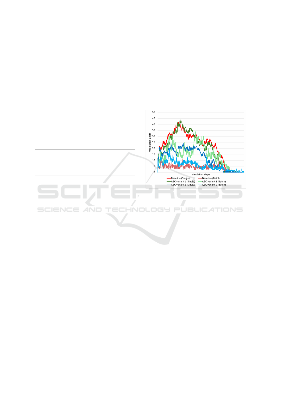
a FIFO order to queues with minimal length. Figure 1
illustrates the influence of each of these algorithms on
the maximum queue length of machines, categorized
by machine type (single and batch).
Figure 1: The impact of each of the three algorithms on
the maximum queue length of machines (single and batch).
As it is observable, ABC variant (2), compared to the other
two, successfully avoided long queues.
As evident from Figure 1, in comparison to the
Baseline algorithm, ABC variant (1) increases the
load on batch machines and disrupts the balance, lead-
ing to an increase in the queue length of batch ma-
chines while the queue length of single machines re-
mains unchanged. On the other hand, ABC variant (2)
effectively maintains the system balance and simulta-
neously prevents the formation of long queues.
Also, Figure 2 depicts consistent results regard-
ing the impact of all three algorithms on the percent-
age of idle batch machines that have entered the wait
timer. It is evident from the image that the Baseline
and ABC variant (2) algorithms effectively maintain
the balance of load on all machines. However, ABC
variant (1) failed to maintain this balance.
Qualitative algorithm performance comparison in-
dicated that ABC variant (2) has been relatively suc-
cessful in maintaining system stability. However, be-
sides maintaining system balance, the primary objec-
tive of designing algorithms is also to boost perfor-
mance. The Tables 3, 4 and 5 present the results of
the quantitative performance study of the two algo-
rithms compared to the Baseline algorithm based on
Artificial Bee Colony Algorithm: Bottom-Up Variants for the Job-Shop Scheduling Problem
109

Figure 2: The impact of each of the three algorithms on the
percentage of batch machines that are on a wait timer and
have no complete batch to process. Compared to the two
other algorithms, the imbalance lot processing of ABC vari-
ant (1) resulted in a considerable percentage of machines
entering wait timers.
the defined performance metrics and using the intro-
duced datasets. It’s important to note that due to the
inherently nondeterministic nature of the processes
involved (e.g., the random decision-making of lots in
certain situations), the repetition of experiments was
crucial for obtaining statistically significant results.
Therefore, each experiment was repeated 100 times
across the three scenarios to provide robustness to the
findings. Thus, the reported results in this section rep-
resent averages derived from the multiple runs con-
ducted for each scenario.
Table 3: Results for small scenario (SFAB) indicate that
both ABC variants result in slightly bigger MS and reduce
UTL, but ABC variant (2) significantly improved FF and
TRD.
Baseline ABC 1 Imp % ABC 2 Imp %
MS 10054.5 10367.3 -3.11 10699.8 -6.42
FF 6.256 6.188 1.09 4.472 28.51
TRD 6647.1 6577.3 1.05 4401.2 33.79
UTL 33.945 33.053 -2.63 31.991 -5.76
In all three case studies, the introduced ABC-
based algorithms caused deterioration in both MS and
machine UTL. This was even worse for ABC-variant
(2). On the other hand, although ABC-variant (1)
could not improve the other two metrics, FF and TRD,
ABC-variant (2) considerably improved on these two
metrics and in all cases.
The analysis of algorithm performance across
three different case sizes, namely small, medium, and
large, serves as a testament to the stability and de-
pendability of these algorithms. While ABC variant
Table 4: Results for medium scenario (MFAB) exhibit the
behavior of the algorithm similar to the SFAB case.
Baseline ABC 1 Imp % ABC 2 Imp %
MS 4559.3 4873 -6.88 4996.5 -9.59
FF 3.084 3.113 -0.93 2.655 13.9
TRD 2358 2388.4 -1.29 1873.2 20.56
UTL 21.514 20.902 -2.84 20.075 -6.69
(1) may not exhibit a substantial improvement in per-
formance, it consistently maintains its stability across
all case sizes. Conversely, the findings highlight that
the impressive performance of ABC variant (2) is not
contingent upon the specific case or its size. This sug-
gests that ABC variant (2) is robust and adaptable.
Table 5: Results for large scenario (LFAB) exhibit match-
ing and reliable behavior of the two proposed algorithms
compared to the Baseline algorithm.
Baseline ABC 1 Imp % ABC 2 Imp %
MS 5933.9 6255.37 -5.42 6767.2 -14.04
FF 3.353 3.337 0.47 2.709 19.2
TRD 2976.6 2955.6 0.71 2157.3 27.52
UTL 21.944 20.451 -6.81 19.59 -10.73
Overall results imply that ABC2 effectively en-
hances the efficiency of FAB in low-level terms and
for individual lots (as evidenced by improvements in
FF and TRD). Still, it doesn’t substantially impact the
overall production time (MS) at a high level. The
reduced UTLs confirm this interpretation. In other
words, by utilizing ABC2, the lengths of machines’
queues are shortened since lots are prioritized based
on minimum waiting time, resulting in lower FF and
TRD. However, ABC2 only looks ahead for lots’
waiting times. It does not consider the later availabil-
ity of lots for machines, so the chance that a machine
gets no lot for a while increases, resulting in lower
UTL and, thus, a higher MS due to the increased idle
machines.
5 CONCLUSION AND FUTURE
WORK
In summary, this study explored the application of the
two versions of the Artificial Bee Colony (ABC) al-
gorithm on the JSSP in the semiconductor industry.
While the first variant does not provide noticeable
improvements, studying its behavior helped us to de-
velop the second variant by avoiding the weaknesses
of the previous one and focusing on the refinement.
SIMULTECH 2024 - 14th International Conference on Simulation and Modeling Methodologies, Technologies and Applications
110

As a result, ABC variant (2) performs consistently
well across different cases, highlighting its versatility.
These findings underline the importance of balancing
stability and adaptability in algorithm design for ef-
fective scheduling in complex manufacturing settings.
Further research could explore different parameters of
ABC variant (2), including look ahead and emphasiz-
ing coef. Furthermore, the role and effectiveness of
scout bees in the system can be investigated.
ACKNOWLEDGEMENT
This work was performed in the course of project
SwarmIn supported by FFG under contract number
894072.
REFERENCES
Alvarado-Iniesta, A., Garcia-Alcaraz, J. L., Rodriguez-
Borbon, M. I., and Maldonado, A. (2013). Optimiza-
tion of the material flow in a manufacturing plant by
use of artificial bee colony algorithm. Expert Systems
with Applications, 40(12):4785–4790.
Gao, K., Cao, Z., Zhang, L., Chen, Z., Han, Y., and
Pan, Q. (2019). A review on swarm intelligence and
evolutionary algorithms for solving flexible job shop
scheduling problems. IEEE/CAA Journal of Automat-
ica Sinica, 6(4):904–916.
Gao, K. Z., Suganthan, P. N., Pan, Q. K., Tasgetiren, M. F.,
and Sadollah, A. (2016). Artificial bee colony algo-
rithm for scheduling and rescheduling fuzzy flexible
job shop problem with new job insertion. Knowledge-
based systems, 109:1–16.
Gupta, M. and Sharma, G. (2012). An efficient modified ar-
tificial bee colony algorithm for job scheduling prob-
lem. International Journal of Soft Computing and En-
gineering (IJSCE), 1(6).
Han, Y.-Y., Pan, Q.-K., Li, J.-Q., and Sang, H.-y. (2012).
An improved artificial bee colony algorithm for the
blocking flowshop scheduling problem. The Interna-
tional Journal of Advanced Manufacturing Technol-
ogy, 60(9-12):1149–1159.
Karaboga, D. and Basturk, B. (2007). A powerful and ef-
ficient algorithm for numerical function optimization:
artificial bee colony (abc) algorithm. Journal of global
optimization, 39(3):459–471.
Karaboga, D., Gorkemli, B., Ozturk, C., and Karaboga, N.
(2014). A comprehensive survey: artificial bee colony
(abc) algorithm and applications. Artificial Intelli-
gence Review, 42(1):21–57.
Khader, A. T., Al-betar, M. A., and Mohammed, A. A.
(2013). Artificial bee colony algorithm, its variants
and applications: a survey. Journal of Theoretical and
Applied Information Technology, 47(2):434–459.
Khatmi, E., Elmenreich, W., Wogatai, K., Schranz, M., Um-
lauft, M., Laure, W., and Wuttei, A. (2019). Swarm in-
telligence layer to control autonomous agents (swilt).
In STAF (Co-Located Events), pages 91–96.
Kumar, S., Sharma, V. K., and Kumari, R. (2014). A
novel hybrid crossover based artificial bee colony al-
gorithm for optimization problem. arXiv preprint
arXiv:1407.5574.
Lawler, E. L., Lenstra, J. K., Kan, A. H. R., and Shmoys,
D. B. (1993). Sequencing and scheduling: Algorithms
and complexity. Handbooks in Operations Research
and Management Science, 4:445–522.
Schranz, M., Di Caro, G. A., Schmickl, T., Elmenreich, W.,
Arvin, F., S¸ekercio
˘
glu, A., and Sende, M. (2021a).
Swarm intelligence and cyber-physical systems: con-
cepts, challenges and future trends. Swarm and Evo-
lutionary Computation, 60:100762.
Schranz, M., Umlauft, M., and Elmenreich, W. (2021b).
Bottom-up job shop scheduling with swarm intelli-
gence in large production plants. In Proceedings of
the 11th International Conference on Simulation and
Modeling, Methodolgies, Technologies and Applica-
tions (SIMULTECH), pages 327–334.
Sharma, N., Sharma, H., and Sharma, A. (2018). Beer froth
artificial bee colony algorithm for job-shop scheduling
problem. Applied Soft Computing, 68:507–524.
Umlauft, M., Gojkovic, M., Harshina, K., Majbour, K.,
and Schranz, M. (2023a). Bees, bats and glow-
worms: Swarm algorithms for optimizing industrial
plants from the bottom-up. In International Confer-
ence on Agents and Artificial Intelligence, pages 3–25.
Springer.
Umlauft, M., Gojkovic, M., Harshina, K., and Schranz, M.
(2023b). Bottom-up bio-inspired algorithms for opti-
mizing industrial plants. In International Conference
on Agents and Artificial Intelligence (ICAART), pages
59–70.
Umlauft, M., Schranz, M., and Elmenreich, W. (2022).
Simulation of swarm intelligence for flexible job-shop
scheduling with swarmfabsim: Case studies with arti-
ficial hormones and an ant algorithm. In International
Conference on Simulation and Modeling Methodolo-
gies, Technologies and Applications, pages 133–155.
Springer.
Yao, B. Z., Yang, C. Y., Hu, J. J., Yin, G. D., and Yu, B.
(2010). An improved artificial bee colony algorithm
for job shop problem. In Applied Mechanics and Ma-
terials, volume 26, pages 657–660. Trans Tech Publ.
Yurtkuran, A. and Emel, E. (2014). A modified artificial bee
colony algorithm for-center problems. The Scientific
World Journal, 2014.
Zhang, G., Shao, X., Li, P., and Gao, L. (2009). An effec-
tive hybrid particle swarm optimization algorithm for
multi-objective flexible job-shop scheduling problem.
Computers & Industrial Engineering, 56(4):1309–
1318.
Artificial Bee Colony Algorithm: Bottom-Up Variants for the Job-Shop Scheduling Problem
111