Privacy-Preserving Big Hierarchical Data Analytics via Co-Occurrence
Analysis
Alfredo Cuzzocrea
1,2 a
and Selim Soufargi
1 b
1
iDEA Lab, University of Calabria, Rende, Italy
2
Department of Computer Science, University of Paris City, Paris, France
Keywords:
Big Data, Privacy-Preserving Big Data, Big Hierarchical Data, Co-Occurrence Analysis, Multidimensional
Big Data Analytics, Privacy-Preserving Multidimensional Big Data Analytics.
Abstract:
Nowadays, Big Data Analytics is gaining the momentum in both the academic and industrial research com-
munities. In this context, the issue of performing such a critical process under tight privacy-preservation con-
straints plays the critical role of “enabling technology”. This paper, by perfectly aligning with the depicted
paradigm, introduces and experimentally assesses Drill-CODA, an innovative framework that combines drill-
across multidimensional big data analytics and co-occurrence analysis to finally achieve privacy-preservation
during the analytical phase.
1 INTRODUCTION
Merging privacy-preservation and big data analytics
(e.g., (Ram Mohan Rao et al., 2018; Tran and Hu,
2019)) is a first-quality research area that is gaining
the attention from both the academic and industrial
research communities. Indeed, while big data analyt-
ics (Russom, 2011; Tsai et al., 2015) offers noticeable
tools for discovering hidden patterns and knowledge,
severe privacy breaches are still possible, especially
when related to personal information. Aggregation
is a common practice to achieve privacy-preserving
data analytics (e.g., (Singh and Kumar, 2023; Wei
et al., 2024)) since aggregates remove details over
personal data. This research line, in fact, has also
originated a long series of research proposals in the
context of privacy-preserving OLAP (e.g., (Agrawal
et al., 2005)).
In the so-delineated research context, big hierar-
chical data (e.g., (Cuzzocrea et al., 2005; Ouazzani
et al., 2021)) play a leading role, since they occur in a
wide collection of application scenarios, ranging from
censor data to logistic data, from geographic data to
biological data, from sensor data to healthcare data,
and so forth. It is worthy to consider that, in all these
settings, big data analytics is a top-notch tool that is
capable of enabling real actionable knowledge pro-
a
https://orcid.org/0000-0002-7104-6415
b
https://orcid.org/0009-0000-5476-9403
cessing in the vest of a significant and valuable add-on
for emerging applications.
This paper, by perfectly aligning with the de-
picted paradigm, introduces and experimentally as-
sesses Drill-CODA, an innovative framework that
combines drill-across multidimensional big data an-
alytics and co-occurrence analysis to finally achieve
privacy-preservation during the analytical phase. In
Drill-CODA, the usage of co-occurrence analysis
(e.g., (Honda et al., 2015; Wu et al., 2021)) combined
with aggregates allows us to achieve an effective and
powerful anonymization effect over big hierarchical
data. The embedded drill-across query layer is used
to magnify the capabilities of multidimensional big
data analytics tools.
Figure 1 shows the Drill-CODA framework data
processing workflow. It includes several layers/steps
according to which input raw data are pre-processed
at the pre-processing layer, even in order to dis-
cover the hidden hierarchies and to prepare them
for the further co-occurrence processing. In the
co-occurrence layer, co-occurrence analysis is per-
formed, also to achieve the desired privacy-preserving
effect (e.g., (Wang et al., 2018; Wang et al., 2020)).
After this step, transformed co-occurrence data are
aggregated according to their discovered hierarchies
and a multidimensional representation is thus ob-
tained. Suitable integrated cubes are consequently
built and stored at this level. Finally, on top of the lat-
ter data cubes, a proper layer of drill-across queries
Cuzzocrea, A. and Soufargi, S.
Privacy-Preserving Big Hierarchical Data Analytics via Co-Occurrence Analysis.
DOI: 10.5220/0012767800003756
Paper published under CC license (CC BY-NC-ND 4.0)
In Proceedings of the 13th International Conference on Data Science, Technology and Applications (DATA 2024), pages 93-103
ISBN: 978-989-758-707-8; ISSN: 2184-285X
Proceedings Copyright © 2024 by SCITEPRESS – Science and Technology Publications, Lda.
93

is executed in the vest of baseline tool for comput-
ing the final privacy-preserving multidimensional big
data analytics (e.g., (Cuzzocrea, 2023)).
2 ANATOMY AND DATA
PROCESSING STEPS OF
DRILL-CODA
Here, we provide a description of the Drill-CODA
steps: pre-processing, co-occurrence analysis, multi-
dimensional aggregation, and drill-across querying.
In the Drill-CODA pre-processing step, the
input hierarchical big datasets in S are treated
for preparation for the next steps of the whole
technique. First, we focus the attention on the
anatomy of these datasets. Being hierarchical in
nature, given a dataset S
j
∈ S, some attributes
W (S) = {A
k
0
, A
k
1
, . . . , A
k
|W (S )|−1
} ∈ S
j
play the role
of dimensions while some other attributes M (S ) =
{A
h
0
, A
h
1
, . . . , A
h
|M (S )|−1
} ∈ S
j
, such that k
u
̸= h
l
∀u∧l,
play the role of measures related to those dimensions.
Given a dimension A
k
u
∈ W (S), a dimensional hi-
erarchy H (A
k
u
) is defined on top of it, as follows:
H (A
k
u
) = {l
A
k
u
,0
, l
A
k
u
,1
, . . . , l
A
k
u
,|H (A
k
u
)|−1
}, such that
l
A
k
u
,q
models a hierarchical level of H (A
k
u
), with q ∈
{0, 1, . . . , DEPT H(H (A
k
u
))−1}, where DEPT H is a
multidimensional operator that retrieves the depth of
the hierarchy H (A
k
u
). However, as it will be clearer
through the paper, while we keep in our model to re-
spect the property of autonomicity, we do not process
neither use the measures of datasets S
j
∈ S directly,
since our framework is oriented to more advanced an-
alytics.
In the pre-processing step, given a dataset
S
j
∈ S, we define: (i) a set of target at-
tributes of interest for the analysis, namely T
S
j
=
{T
S
j
,0
, T
S
j
,1
, . . . , T
S
j
,|T
S
j
|−1
}, and the respective set
of attribute values of interest for the analy-
sis, namely V
S
j
= {V
S
j
,0
, V
S
j
,1
, . . . , V
S
j
,|V
S
j
|−1
}, such
T
S
j
,k
= V
S
j
,k
, ∀k ∈ {0, 1, . . . , |T
S
j
| − 1 = |V
S
j
| − 1};
(ii) a specific aggregate operator selected in the
set AO = {SUM, COUNT, MIN, MAX, AVG}, which
applies on top of the target attributes in T
S
j
;
(iii) a set of functional attributes with respect to
which the target attributes are analyzed, namely
F
S
j
= {F
S
j
,0
, F
S
j
,1
, . . . , F
S
j
,|F
S
j
|−1
}, such that T
S
j
,k
̸=
F
S
j
,h
, ∀k ̸= h.
Based on these definitions, we project S
j
by tar-
get attributes in T
S
j
, and then we filter the obtained
projected dataset by means of values in V
S
j
. After
that, we apply the given aggregate operator in AO
and we aggregate data of target attributes along all
the hierarchies of dimensions in W (S
j
). Of course,
we aggregate the functional attributes in F
S
j
as well.
Formally, we denote the pre-processed dataset de-
rived from S
j
as S
PP
j
, and we construct the set S
PP
=
{S
PP
0
, S
PP
1
, . . . , S
PP
|S
PP
|−1
}.
In the Drill-CODA co-occurrence analysis step,
the final goal is that of obtaining the privacy-
preservation effect, since we apply a kind of co-
occurrence-based anonymization technique that takes
advantage from the multidimensional nature of tar-
get data. Before going into details, to become con-
vinced about the approach, consider the following
toy example. Let D
i,H
and D
j,H
be two big health-
care datasets that store patient events about diseases,
treatments, therapies and so forth, being the lat-
ter all sensitive data whose privacy should be pre-
served. Here, it is interesting and natural to an-
alyze correlations that may exist among data D
i,H
and D
j,H
, in order, for instance, to discover cross-
therapies performed by different hospitals over the
same diseases, in order to ameliorate the effective-
ness of combined therapies, perhaps obtained from
the merging of therapies of different hospitals. In this
case, let Location and Time be two co-occurrence
attributes, both belonging to the schemes of D
i,H
and D
j,H
, respectively. Given a specific death
event, for instance caused by cancer, it is possible to
compute two different co-occurrence datasets from
D
i,H
and D
j,H
, namely CO[D
i,H
, D
j,H
, Location]
and C O[D
i,H
, D
j,H
, Time], respectively, such that
C O[D
i,H
, D
j,H
, Location] stores the death events of
D
i,H
and D
j,H
that refer to the same Location, while
C O[D
i,H
, D
j,H
, Time] stores the death events of D
i,H
and D
j,H
that refer to the same Time, respectively. It
should be noted that both the two co-occurrence at-
tributes Location and Time model specific hierarchi-
cal levels of certain hierarchies associate to dimen-
sions in both D
i,H
and D
j,H
, respectively. More-
over, the co-occurrence analysis provides us with the
desiderata privacy-preservation effect due to the fact
that, when abstracted to the Time level, e.g. Year, and
the Location level, e.g. Country, individual data are
anonymized while aggregate data still suffice to the
big data analytics purposes.
Formally, given the set of pre-processed hierar-
chical big datasets S
PP
= {S
PP
0
, S
PP
1
, . . . , S
PP
|S
PP
|−1
}
and a set of common co-occurrence attributes
A
S,CO
= {A
S,CO,0
, A
S,CO,1
, . . . , A
S,CO,|A
S,CO
|−1
} ∈
S
j
∈ S, such that A
S,CO,k
∈ S
PP
j
, ∀S
PP
j
∈
S
PP
, ∀k ∈ {0, 1, . . . , |A
S,CO
| − 1}, we gener-
ate |A
S,CO
| − 1 co-occurrence datasets, namely
C O
S,CO
= {C
S,CO,0
, C
S,CO,1
, . . . , C
S,CO,|A
S,CO
|−1
},
DATA 2024 - 13th International Conference on Data Science, Technology and Applications
94

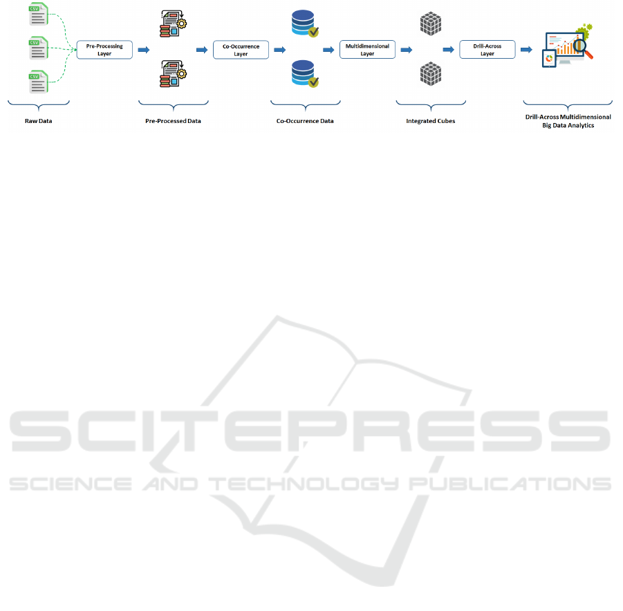
Figure 1: The Drill-CODA Framework Data Processing Workflow.
such that each dataset C
S,CO,k
∈ C O
S,CO
is defined as
follows:
C
S,CO,k
= {A
S,CO,k
, ⟨F
S
j
,h
, {AO
0
(T
S
j
,0
), AO
1
(T
S
j
,1
), . . . ,
AO
|T
S
j
|−1
(T
S
j
,|T
S
j
|−1
)}⟩},
∀k ∈ {0, 1, . . . , |A
S,CO
| − 1}
(1)
such that: (i) A
S,CO,k
, where k ∈ {0, 1, . . . , |A
S,CO
| −
1} denotes a co-occurrence attribute; (ii) F
S
j
,h
, where
h ∈ {0, 1, . . . , |F
S
j
|−1} denotes a functional attribute;
(iii) AO
z
, where z ∈ {0, 1, . . . , |AO| − 1}, denotes an
aggregate operator selected from the set AO.
To give an example, consider the schema of
the first co-occurrence dataset, defined as follows:
{Year, ⟨Gender, COUNT (SkinCancer), COUNT
(LungCancer), COU NT (Diabetes Type1), COUNT (
Diabetes Type2)⟩}. A possible instance is the
following one: {2022, {⟨F-Cancer, 35, 74⟩, ⟨M-
Cancer, 37, 58⟩, ⟨M-Diabetes, 27, 51⟩, ⟨F-Diabetes,
43, 68⟩}, which models the event that, during 2022,
with no reference to the location, (i) a total of 109
female (F) patients died by cancer, specifically 35
of SkinCancer and 74 of LungCancer; (ii) a total of
95 male (M) patients died by cancer, specifically 37
of SkinCancer and 58 of LungCancer; (iii) a total of
78 male (M) patients died by diabetes, specifically
27 of DiabetesType 1 and 51 of Diabetes Type2;
(iv) a total of 111 female (F) patients died by
diabetes, specifically 43 of Diabetes Type1 and 68 of
Diabetes Type2.
Similarly, consider the schema of the sec-
ond co-occurrence dataset, defined as follows:
{Country, ⟨Gender, COUNT (SkinCancer), COUNT (
LungCancer), COUNT (Diabetes Type1), COUNT (
Diabetes Type2)⟩}. A possible instance is the
following one: {France, {⟨M-Cancer, 28, 61⟩, ⟨F-
Cancer, 35, 74⟩, ⟨M-Diabetes, 30, 63⟩, ⟨F-Diabetes,
43, 68⟩}, which the event that, in France, with no ref-
erence to the time, (i) a total of 89 male (M) patients
died by cancer, specifically 28 of SkinCancer and 61
of LungCancer; (ii) a total of 109 female (F) patients
died by cancer, specifically 35 of SkinCancer and 74
of LungCancer; (iii) a total of 93 male (M) patients
died by diabetes, specifically 30 of Diabetes Type1
and 63 of Diabetes Type2; (iv) a total of 111 female
(F) patients died by diabetes, specifically 43 of
Diabetes Type1 and 68 of Diabetes Type2.
From the examples above, it should be explicitly
noted that, in our co-occurrence dataset, we group-by
the aggregate values of the target attributes by means
of the values of the functional attributes (e.g., F-
Cancer: aggregate values of COU NT (SkinCancer)
and COUNT (LungCancer) are grouped-by the gen-
der of the patient F). This is due to the fundamental
definition of co-occurrence analysis.
In the Drill-CODA multidimensional aggre-
gation step, ad-hoc OLAP data cubes are built
from the input co-occurrence datasets computed
at the previous step (the co-occurrence analysis
step). Given the input co-occurrence datasets
C O
S,CO
= {C
S,CO,0
, C
S,CO,1
, . . . , C
S,CO,|A
S,CO
|−1
},
we compute |A
S,CO
| − 1 multidimensional OLAP
data cubes as belonging to the set DC(C O
S,CO
) =
{DC
S,CO,0
, DC
S,CO,1
, . . . , DC
S,CO,|DC(CO
S,CO
)|−1
},
where |A
S,CO
| − 1 = |DC(C O
S,CO
)| − 1, such that
each data cube DC
S,CO,k
∈ DC(C O
S,CO
) is defined
as follows:
DC
S,CO,k
= ⟨{A
S,CO,0
, A
S,CO,1
, . . . , A
S,CO,|A
S,CO
|−1
},
{AO
0
(T
S
j
,0
), AO
1
(T
S
j
,1
), . . . , AO
|T
S
j
|−1
(T
S
j
,|T
S
j
|−1
)}⟩,
∀k ∈ {0, 1, . . . , |A
S,CO
| − 1}
(2)
such that: (i) A
S,CO,k
, where k ∈ {0, 1, . . . , |A
S,CO
| −
1} denotes a dimension (which corresponds to
a co-occurrence attribute); (ii) AO
z
, where z ∈
{0, 1, . . . , |AO| − 1}, denotes an aggregate operator
selected from the set AO; (iii) T
S
k
, where k ∈
{0, 1, . . . , |T
S
j
| − 1}, denotes a target attribute of in-
terest for the analysis. It should be noted, here, that:
(i) each OLAP data cube DC
S,CO,k
∈ DC(C O
S,CO
) is,
formally, a multiple-measure data cube; (ii) the num-
ber of measures, which corresponds to the number of
attributes of interest for the analysis, is the same for
each OLAP data cube DC
S,CO,k
∈ DC (CO
S,CO
).
To give an example, consider a simple two-
dimensional model. Here, let ⟨{Year, Gender-
Privacy-Preserving Big Hierarchical Data Analytics via Co-Occurrence Analysis
95

Disease}, {COU NT ({SkinCancer, LungCancer}),
COUNT ({Diabetes Type1, Diabetes Type 2})}⟩ be
the schema of the first (two-dimensional) OLAP
data cube. A possible data cube cell instance is the
following one: ⟨2020, M-Cancer⟩ = ⟨32, 69⟩, which
models the event that, during 2020, with no reference
to the location, a total number of 32 male (M) patient
died by SkinCancer and a total number of 69 male
(M) patient died by LungCancer.
Similarly, let ⟨{Country, Gender-Disease},
{COUNT ({SkinCancer, LungCancer}), COU NT ({
Diabetes Type1, Diabetes Type 2})}⟩ be the schema
of the second (two-dimensional) OLAP data cube.
A possible data cube cell instance is the following
one: ⟨Italy, F-Diabetes⟩ = ⟨31, 55⟩, which models
the event that, in Italy, with no reference to the
time, a total number of 31 female (F) patient died by
Diabetes Type1 and a total number of 55 female (F)
patient died by Diabetes Type2.
In the Drill-CODA drill-across query-
ing step, given the collection of OLAP data
cubes DC (CO
S,CO
) = {DC
S,CO,0
, DC
S,CO,1
, . . . ,
DC
S,CO,|DC(CO
S,CO
)|−1
}, computed at the previous
step (the multidimensional aggregation step), we gen-
erate, for each data cube DC
S,CO,k
∈ DC(C O
S,CO
), a
full-dimensional drill-across query Q
Q ,CO,k
, defined
as follows:
Q
S,CO,k
= ⟨{[A
S,CO,0
[0] : A
S,CO,0
[|A
S,CO,0
| − 1]],
[A
S,CO,1
[0] : A
S,CO,1
[|A
S,CO,1
| − 1]],
. . . ,
[A
S,CO,|A
S,CO
|−1
[0] : A
S,CO,|A
S,CO
|−1
[|A
S,CO,|A
S,CO
|−1
| − 1]]}, AO
k
(T
S
j
,k
)⟩
∀k ∈ {0, 1, . . . , |DC (CO
S,CO
)| − 1}
(3)
such that: (i) A
S,CO,k
, where k ∈ {0, 1, . . . , |A
S,CO
| −
1} denotes a dimension of DC
S,CO,k
(which corre-
sponds to a co-occurrence attribute); (ii) A
S,CO,k
[0]
denotes the first dimensional member in A
S,CO,k
;
(iii) A
S,CO,k
[|A
S,CO,k
| − 1] denotes the last dimen-
sional member in A
S,CO,k
; (iv) AO
z
, where z ∈
{0, 1, . . . , |AO| − 1}, denotes an aggregate opera-
tor selected from the set AO; (v) T
S
k
, where k ∈
{0, 1, . . . , |T
S
j
| − 1}, denotes a target attribute of in-
terest for the analysis. It should be noted that the full-
dimensional drill-across query Q
S,CO,k
spans all the
dimensions of DC
S,CO,k
along all their dimensional
domains.
By iterating the described procedure for each
data cube DC
S,CO,k
∈ DC(C O
S,CO
), we obtain the
so-called full-dimensional drill-across query set
Q
C O
(S) = {Q
Q ,CO,0
, Q
Q ,CO,1
, . . . , Q
Q ,CO,|Q
C O
(S)|−1
}.
After that, each drill-across query Q
Q ,CO,k
∈
Q
C O
(S) is executed against all the collec-
tion of OLAP data cubes DC (CO
S,CO
) =
{DC
S,CO,0
, DC
S,CO,1
, . . . , DC
S,CO,|DC(CO
S,CO
)|−1
},
thus finally originating the full-dimensional corre-
lation set D
C O
(S). From Section 1, remind that
D
C O
(S) stores collections of correlated aggregates.
To give an example, consider a simple two-
dimensional model. Here, let ⟨{Year, Gender-
Disease}, {COU NT ({SkinCancer, LungCancer}),
COUNT ({Diabetes Type1, Diabetes Type 2})}⟩ be
the schema of the first (two-dimensional) OLAP data
cube, and ⟨{Country, Gender-Disease}, {COUNT (
{SkinCancer, LungCancer}), COU NT ({Diabetes
Type 1, Diabetes Type 2})}⟩ be the schema of
the second (two-dimensional) OLAP data cube,
respectively. Let ⟨{[2020 : 2023], [M-Cancer : F-
Diabetes]}, SUM⟩ be the input drill-across query
against the two data cubes. The answer to the query
is ⟨358, 734⟩. The latter models the event that, from
2020 to 2023, a total number of 358 patients, with no
reference to their sex, died by Cancer (including both
SkinCancer and LungCancer), and a total number
of 734 patients, with no reference to their sex, died
by Diabetes (including both Diabetes Type1 and
Diabetes Type2).
3 A COMPLETE DRILL-CODA
CASE STUDY
In this Section, a complete example of Drill-CODA
data processing workflow steps (see Section 1) is pre-
sented. For the sake of clarity and simplicity, we con-
sider a simple but effective two-dimensional model. It
is also worth noting that our approach is also valid for
multidimensional models, as highlighted in Section 1.
Specifically, our attention is directed toward the in-
troduction of two synthetic hierarchical datasets, de-
noted as D
1
and D
2
, designed to store disease-related
information. Each record within these datasets rep-
resents a death event related to a particular disease.
Figure 2 and Figure 3 show the structure and example
record of D
1
and D
2
, respectively.
For each dataset under consideration, we estab-
lish multidimensional hierarchies that provide a struc-
tured framework for organizing and analyzing the
data. Specifically, both datasets feature two key hi-
erarchies: a temporal hierarchy denoted as H (T ) =
Day ← Month ← Year, capturing the temporal as-
pects of the data, and a spatial hierarchy denoted as
H (S) = City ← Region ← Country, representing the
geographical dimensions. Beyond these fundamen-
tal hierarchies, additional attributes further enrich the
datasets: (i) the attribute Gender serves to categorize
DATA 2024 - 13th International Conference on Data Science, Technology and Applications
96

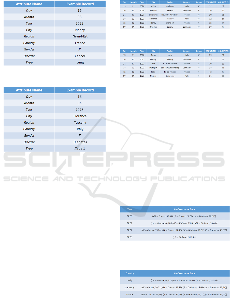
Figure 2: Structure and Example Record of the Dataset D
1
of the Case Study.
Figure 3: Structure and Example Record of the Dataset D
2
of the Case Study.
and model the gender of the patient; (ii) the attribute
Disease encapsulates information about the disease
affecting the patient; (iii) the attribute Type models
the specific type of disease affecting the patient.
Indeed, the initial stage of Drill-CODA is devoted
to pre-processing the input datasets, as described in
Section 1. The functional property for D
1
and D
2
in
our case study is Gender, whereas the target attribute
is Disease. For our case study, we have used COU NT
as the aggregate operator. As a result, we utilize the
values of Cancer for the attribute Disease and Skin
and Lung for the (associated) attribute Type in D
1
.
Similarly, we use the values Type 1 and Type 2 of
the (related) parameter Type and the value Diabetes
of the attribute Disease to filter the data in D
2
. In
terms of the aggregate operator, we use COUNT
for the target attributes of both D
1
and D
2
. Fig-
ure 4 shows the pre-processing for D
1
that generates
the dataset D
1
[Cancer, {Skin, Lung}, COU NT ] (here,
SC denotes the attribute value Skin and LC denotes
the attribute value Lung, respectively), while Fig-
ure 5 shows the pre-processing for D
2
that generates
the dataset D
2
[Diabetes, {Type1, Type2}, COUNT ]
(here, T 1 denotes the attribute value Type1 and T 2
denotes the attribute value Type 2, respectively).
Figure 4: Dataset D
1
[Cancer, {Skin, Lung}, COUNT ] after
the Pre-Processing Step over D
1
.
Figure 5: D
2
[Diabetes, {Type 1, Type 2}, COUNT ] after the
Pre-Processing Step over D
2
.
The Drill-CODA approach requires the co-
occurrence analysis to be conducted following the
pre-processing stage (see Section 1). In Section 2,
pre-processed datasets are used to find frequent co-
occurrence attributes based on analytic goals, result-
ing in relevant co-occurrence datasets. Specifically,
in this case study and for the purpose of ensuring high
privacy-preservation, we select Year and Country as
co-occurrence attributes, according to the guidelines
discussed in Section 2. Figure 6 and Figure 7
show the co-occurrence dataset originated from the
co-occurrence analysis on the (pre-processed)
datasets D
1
[Cancer, {Skin, Lung}, COU NT ]
and D
2
[Diabetes, {1, 2}, COU NT ] over
Year, and the (pre-processed) datasets
D
1
[Cancer, {Skin, Lung}, COU NT ] and
D
2
[Diabetes, {1, 2}, COU NT ] over Country, re-
spectively.
Figure 6: Co-Occurrence Dataset Generated from
Datasets D
1
[Cancer, {Skin, Lung}, COUNT ] and
D
2
[Diabetes, {1, 2}, COUNT ] over Year.
Figure 7: Co-Occurrence Dataset Generated from
Datasets D
1
[Cancer, {Skin, Lung}, COUNT ] and
D
2
[Diabetes, {1, 2}, COUNT ] over Country.
Privacy-Preserving Big Hierarchical Data Analytics via Co-Occurrence Analysis
97

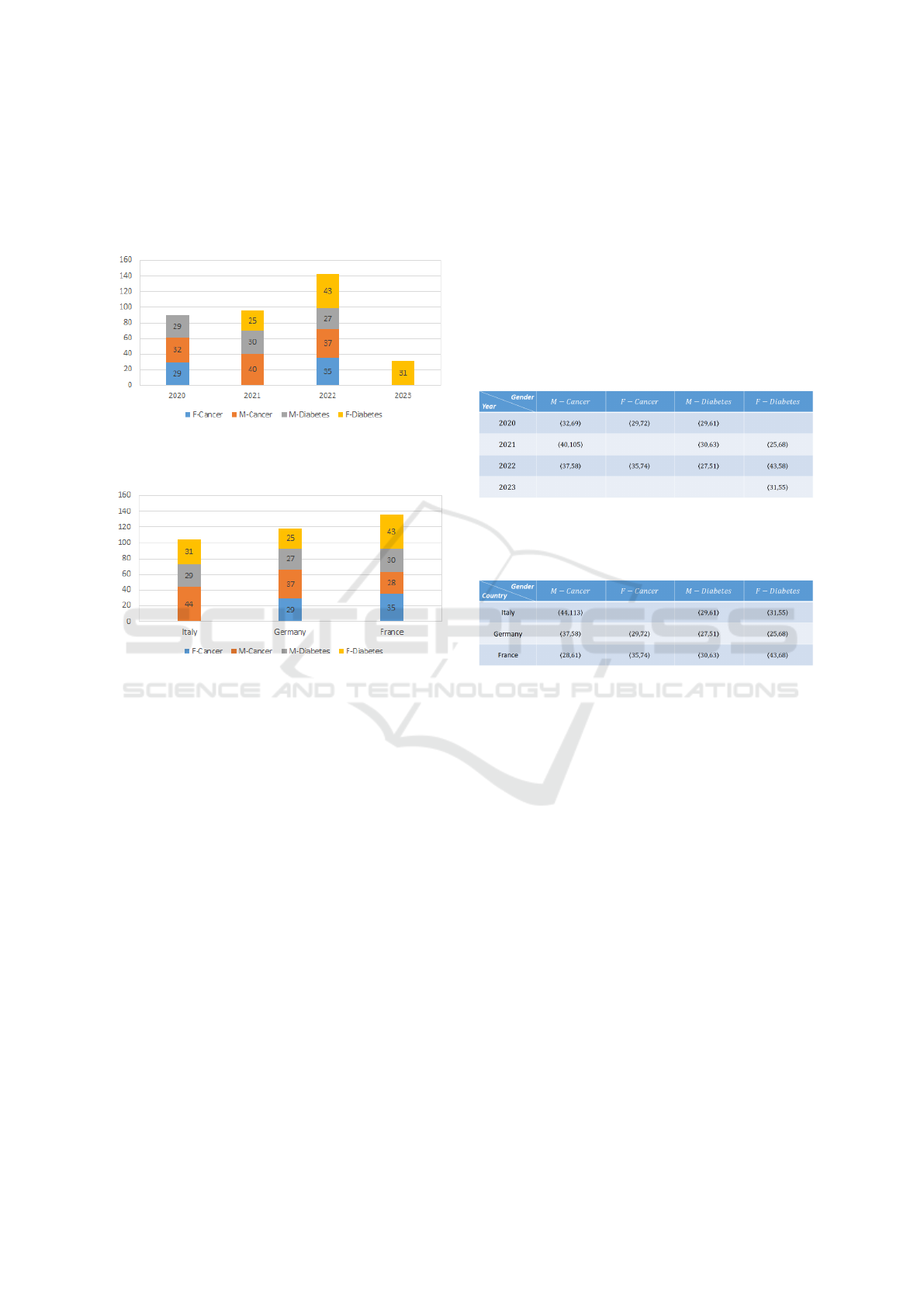
Figure 8 presents the Time co-occurrence analyt-
ics over the co-occurrence dataset shown in Figure 6,
while Figure 9 presents the Location co-occurrence
analytics over the co-occurrence dataset shown in Fig-
ure 7, respectively.
Figure 8: Time Co-Occurrence Analytics over Co-
Occurrence Dataset of Figure 6.
Figure 9: Location Co-Occurrence Analytics over Co-
Occurrence Dataset of Figure 7.
Figure 8 and Figure 9 show that the count of
deaths per gender and per disease on the Y axis and
either the year or the location, respectively, on X
axis. Detailed count per month (see Figure 8) or per
city (see Figure 9) is therefore not displayed, and the
data are anonymized up to the highest hierarchical
level of the time/location attributes. The highest lo-
cation co-occurrences has happened in France, with
more than 130 cases across the four possible values
of Gender − Disease attribute, and the least were in
Italy, with roughly a bit more than 100 death cases and
where no female has died of cancer. Whereas for the
time co-occurrences, the highest count of death cases
is registered for the year 2022 and the least count is
registered for the year 2023, where only female death
cases from diabetes were registered.
Following the acquisition of co-occurrence
data, the subsequent step involves computing suit-
able OLAP data cubes for supporting big data
analytics (see Section 1). In our specific case
study, utilizing the two co-occurrence datasets
generated during the preceding stage of Drill-
CODA, we proceed with the creation of two-
dimensional OLAP data cubes. The initial cube,
denoted as A
1
, is defined as A
1
= ⟨{Year, Gender-
Disease}, {COU NT ({Skin, Lung}), COUNT ({Type
1, Type 2})}⟩ (see Figure 10). This data cube
encapsulates the temporal dimension (Year) and
the composite Gender − Disease category. Si-
multaneously, the second OLAP data cube A
2
is defined as A
2
= ⟨{Country, Gender-Disease},
{COUNT ({Skin, Lung}), COU NT ({Type 1, Type2})
}⟩ (see Figure 11), which delves into the geograph-
ical aspect by incorporating the Country dimension
alongside the Gender − Disease attribute.
Figure 10: Two-Dimensional OLAP Data Cube
A
1
= ⟨{Year, Gender-Disease}, {COU NT ({Skin, Lung}),
COUNT ({Type 1, Type 2})}⟩.
Figure 11: Two-Dimensional OLAP Data Cube A
2
=
⟨{Country, Gender-Disease}, {COU NT ({Skin, Lung}),
COUNT ({Type 1, Type 2})}⟩.
As shown in Figure 10 and Figure 11, we can no-
tice that the dimensions of the OLAP data cubes are
ordered according to a certain topological ordering.
This conclusion is influenced by considering the data
organization and OLAP query performance.
Figure 12 shows the Time two-dimensional co-
occurrence analytics derived from the OLAP data
cube in Figure 10, while Figure 13 shows the
Location two-dimensional co-occurrence analytics
derived from the OLAP data cube in Figure 11, re-
spectively. Here, for each time/location index (e.g.,
2020 or Germany), we show both values of the cou-
ple of measures representing the count of deaths by
the sub-type of the diseases.
The final goal of our Drill-CODA framework con-
sists of performing and building the full-dimensional
correlation set D
C O
(S) (see Section 1). This latter
is tailored to store sets of correlated aggregates re-
trieved from the execution of a suitable set of drill-
across queries along all the hierarchical dimensions
defined on the input set of hierarchical big datasets S,
DATA 2024 - 13th International Conference on Data Science, Technology and Applications
98

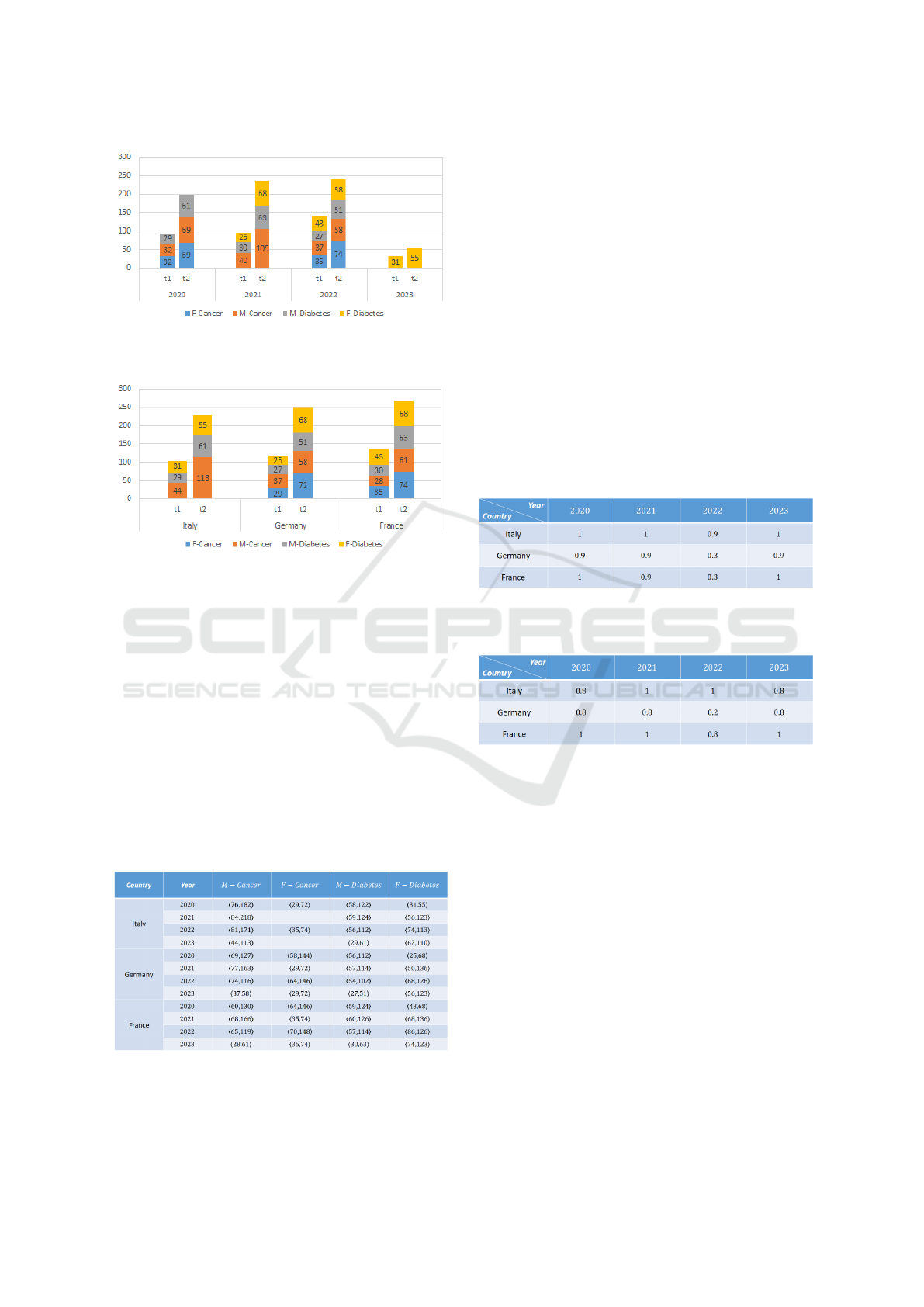
Figure 12: Time Two-Dimensional Co-Occurrence Analyt-
ics derived from the OLAP Data Cube in Figure 10.
Figure 13: Location Two-Dimensional Co-Occurrence An-
alytics derived from the OLAP Data Cube in Figure 11.
taking as input the ad-hoc OLAP data cubes built at
the third step of the Drill-CODA’s methodology.
The full-dimensional correlation set D
C O
(S) is
computed by executing all the sets of admissible full-
dimensional drill-across queries over datasets in S ,
along all their dimensional domains (see Section 2).
Figure 14 shows the full-dimensional correlation set
D
C O
({D
1
, D
2
}) for the running case study.
D
C O
(S), being S = {D
1
, D
2
}, according to what
described in Section 2, is computed by executing
all the set of admissible full-dimensional drill-across
queries over datasets in S, along all their dimensional
domains. Figure 14 shows the full-dimensional corre-
lation set D
C O
({D
1
, D
2
}) for the running case study.
Figure 14: Full-Dimensional Correlation Set
D
C O
({D
1
, D
2
}) for the Running Case Study.
In this research, we conduct a correlation
analysis over the full-dimensional correlation set
D
C O
({D
1
, D
2
}) via two widely used correlation met-
rics (i.e., Pearson correlation coefficient and the
Spearman correlation coefficient) (Corder and Fore-
man, 2014).
Furthermore, for each correlated aggregate pair
⟨M
1
, M
2
⟩ of the full-dimensional correlation set
D
C O
({D
1
, D
2
}), we compute the Pearson correlation
coefficient and the Spearman correlation coefficient in
order to obtain the so-called full-dimensional Pearson
correlation set, denoted by P
C O
({D
1
, D
2
}), and the
so-called full-dimensional Spearman correlation set,
denoted by S
C O
({D
1
, D
2
}), respectively.
Indeed, Figure 15 and Figure 16 show the full-
dimensional Pearson correlation set P
C O
({D
1
, D
2
})
and the full-dimensional Spearman correlation set
S
C O
({D
1
, D
2
}) for the running case study, respec-
tively.
Figure 15: Full-Dimensional Pearson Correlation Set
P
C O
({D
1
, D
2
}) for the Running Case Study.
Figure 16: Full-Dimensional Spearman Correlation Set
S
C O
({D
1
, D
2
}) for the Running Case Study.
4 DRILL-CODA CLOUD-BASED
REFERENCE ARCHITECTURE
In this Section, we introduce the Cloud-based ref-
erence architecture for the proposed Drill-CODA
framework. We start by elucidating the underlying
motivation for a real-world case study of our tech-
nique and highlighting how Drill-CODA can be suc-
cessfully used in the context of big data analytics plat-
forms.
Modern big data analytics applications usually
run on top of massive, large-scale big data reposito-
ries. As a consequence, there is a need for accessing,
processing, and analyzing such repositories via both
well-consolidated big data management and analyt-
Privacy-Preserving Big Hierarchical Data Analytics via Co-Occurrence Analysis
99

ics techniques and well-established Cloud-based big
data processing platforms, such as Hadoop, Spark,
and Kylin.
In reply to these clear requirements, Drill-CODA
must be deployed in a naive big data environment, as
to take advantage of high-computation capabilities,
scalability, virtualization, parallel/distributed execu-
tions, in-memory partial computations, and so forth.
This evidence is stirred-up by the fact that Drill-
CODA mostly processes multidimensional big data,
hence, it can easily incur in the so-called curse of di-
mensionality problem (e.g., (Cuzzocrea et al., 2003)),
meaning that performance of algorithms over multidi-
mensional data decreases when the number of dimen-
sions of input datasets increases. As a consequence,
our study explores the anatomy and the functionalities
of the big-data-aware Drill-CODA deployment. Fig-
ure 17 shows the Cloud-based Drill-CODA reference
architecture.
Co-Occurrence Layer
Pre-Processed Data 2
Pre-Processed Data n
Pre-Processed Data 1
Processed Data 1
Processed Data 2
Processed Data n
Analytical Big Data Warehouse
Drill-CODA Core
Drill-Across Multidimensional
Big Data Analytics
Hadoop Cluster
Pre-Processing Layer
Raw Data 2
Raw Data n
Raw Data 1
Data Source Layer
Data Staging Layer
Cloud Based Analytical Big
Data Warehouse Layer
Big Data Analytics Layer
Drill-Coda Layer
Figure 17: The Cloud-Based Drill-CODA Reference Archi-
tecture.
As shown in Figure 17, the Cloud-based Drill-
CODA reference architecture includes the following
layers:
1. Data Source Layer: In this layer, the original data
sources of our Cloud-based Drill-CODA frame-
work are fed as input to our enabling tool. Data,
as collected from their sources (web, repositories,
and so forth), are used as main entry for our data
flow. Depending on their format and structure,
which should be “unified” for subsequent process-
ing, we apply cleansing and formatting transfor-
mations on them before considering them ready
for the next data staging phase.
2. Pre-Processing Layer. Here, normalized data
sources are pre-processed according to the Drill-
CODA paradigm (see Section 2). This calls for a
pre-processing step to cleanse and reformat data
columns when needed, and above all, the crafting
of data for the respective co-occurrence attributes,
so that a valid drill-down operation could later be
applied to the OLAP cubes to analyze. Also, ag-
gregation along hierarchies is performed.
3. Co-Occurrence Layer. Here, the Co-Occurrence
Layer supports our co-occurrence analysis (see
Section 2). Our main goal through this phase is
to ensure that co-occurrence attributes are present
and allow the creation of a consequent hierarchy
later-on for our multidimensional analysis. The
co-occurrence aggregate data are provided as fi-
nal output.
4. Data Staging Layer. In this layer, we material-
ize the co-occurrence data into suitable data struc-
tures, on top of which multidimensional analysis
is later performed. This step is required to prepare
the data for querying in highly-multidimensional
fashion and make the data (type and format es-
sentially) suitable for deployment onto the data
warehouse solutions.
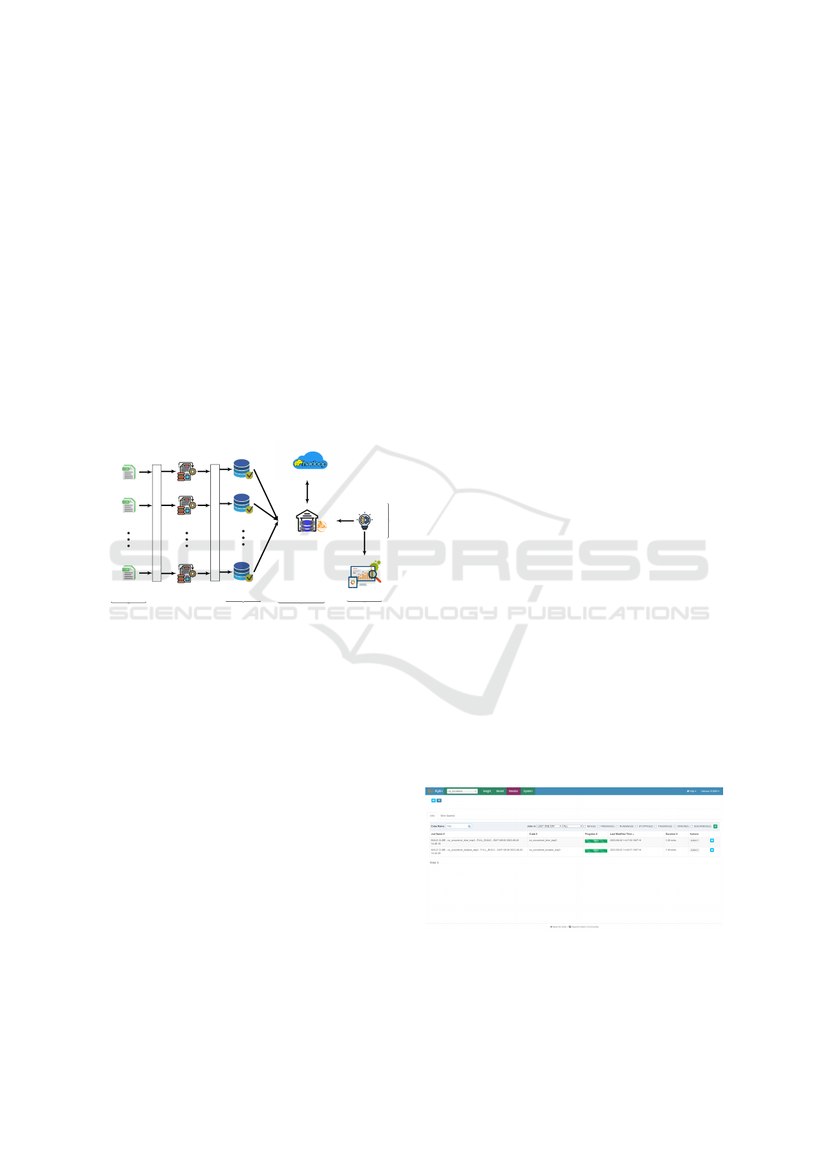
5. Cloud-Based Analytical Big Data Warehouse
Layer. In this layer, thanks to the Kylin OLAP
framework and its interoperability with Hadoop,
multidimensional data are aggregated on top of
staging co-occurrence data in a MapReduce fash-
ion. Indeed, Kylin is a big data platform for
data warehousing and OLAP that integrates a
Spark-based OLAP engine needed for the Hadoop
MapReduce parallel data processing. In fact,
Kylin is capable of integrating, deploying, and
processing a high number of cubes in a concur-
rent manner through Hadoop. In our case study,
we use Kylin MDX to query the cube using Mul-
tidimensional Expressions (MDX). Indeed, after
including the staged data sources and after creat-
ing the data model of the cube as well as the de-
ployment of the cube in Kylin, the tool enables the
querying through MDX using a third-party Busi-
ness Intelligence tool such as Tableau or Excel.
Figure 18 and Figure 19 show the deployment of
cubes in Kylin and Kylin MDX, respectively.
Figure 18: Deployed Cubes in Kylin.
An example of MDX query, we are using the ex-
tract the data from one cube is shown in Figure 20.
DATA 2024 - 13th International Conference on Data Science, Technology and Applications
100

Figure 19: Deployed Cubes in Kylin MDX.
WITH
MEMBER MEASURES.COUNT1 AS [Measures].[Count1]
MEMBER MEASURES.COUNT2 AS [Measures].[Count2]
SELECT { MEASURES.COUNT1, MEASURES.COUNT2 }
ON COLUMNS,
NON EMPTY{(
DRILLDOWNLEVEL({ [Location_Co_Occurence]
.[Hierarchy].[City_Name] }
),[Location_Co_Occurence]
.[Substance_Gender].[Substance_Gender])}
ON ROWS
FROM [location_co_occurence_cube]
Figure 20: MDX Query to Drill-Down from Region →
Country → City.
6. Drill-CODA Layer. In the Drill-CODA Layer, the
core components of Drill-CODA run in order to
derive drill-across multidimensional big data an-
alytics over big co-occurrence aggregate hierar-
chical data, according to the main guidelines pro-
posed by our research (see Section 2).
7. Big Data Analytics Layer. Here, the final desider-
ata big data analytics applies, in order to provide
useful and actionable knowledge from large-scale
big data repositories, mostly by focusing the at-
tention on the full-dimensional correlation pattern
discovery (see Section 3).
5 EXPERIMENTAL ANALYSIS
AND RESULTS
In this Section, we present our experimental assess-
ment of the proposed Drill-CODA framework. This
involves conducting several experimental tests over
large-scale real-life datasets in order to evaluate the
performance and capabilities of the framework.
As regards datasets, we deliberately selected dif-
ferent real-life datasets, as to give more reliability to
the scope and effectiveness of our experimental cam-
paign. In compliance with the primary objectives of
the framework (see Section 2), we perform our evalu-
ation based on co-occurrence analysis.
Figure 21: Time Co-Occurrence Analysis over the Cancer-
Incidence/Mental-Disorders Experimental Setup.
In more details, we focus on the correlation be-
tween cancer incidence and mental disorders. Here,
we used the following real-life datasets: (i) Can-
cer Incidence (CI5Plus): the CI5Plus database con-
tains updated annual incidence rates for 124 selected
populations from 108 cancer registries published in
CI5Plus, for the longest period available (up to 2012),
for all cancers and 28 major types (Organization,
2023); (ii) Mental Disorders: this dataset contains
informative data from Countries across the globe
about the prevalence of mental health disorders, in-
cluding schizophrenia, bipolar disorder, eating disor-
ders, anxiety disorders, drug use disorders, depression
and alcohol use disorders (Devastator, 2023).
In our evaluation, we conduct a co-occurrence
analysis (i.e., time and location co-occurrence) over
the previously described experiment. Here, we dis-
play the findings of our investigation that were gen-
erated using Python/Matplotlib library. Therefore,
let us notice that co-occurrence data is plotted in an
anonymized manner, since only the Year (Region,
respectively) attribute numbers are depicted, being
those attributes the higher level of the time and the
location hierarchies.
For the time co-occurrence analysis (see Fig-
ure 21), a spike in cancer incidence is noticeable start-
ing from year 1998, while mental disorders count-
ing was highly fluctuating for both men and women.
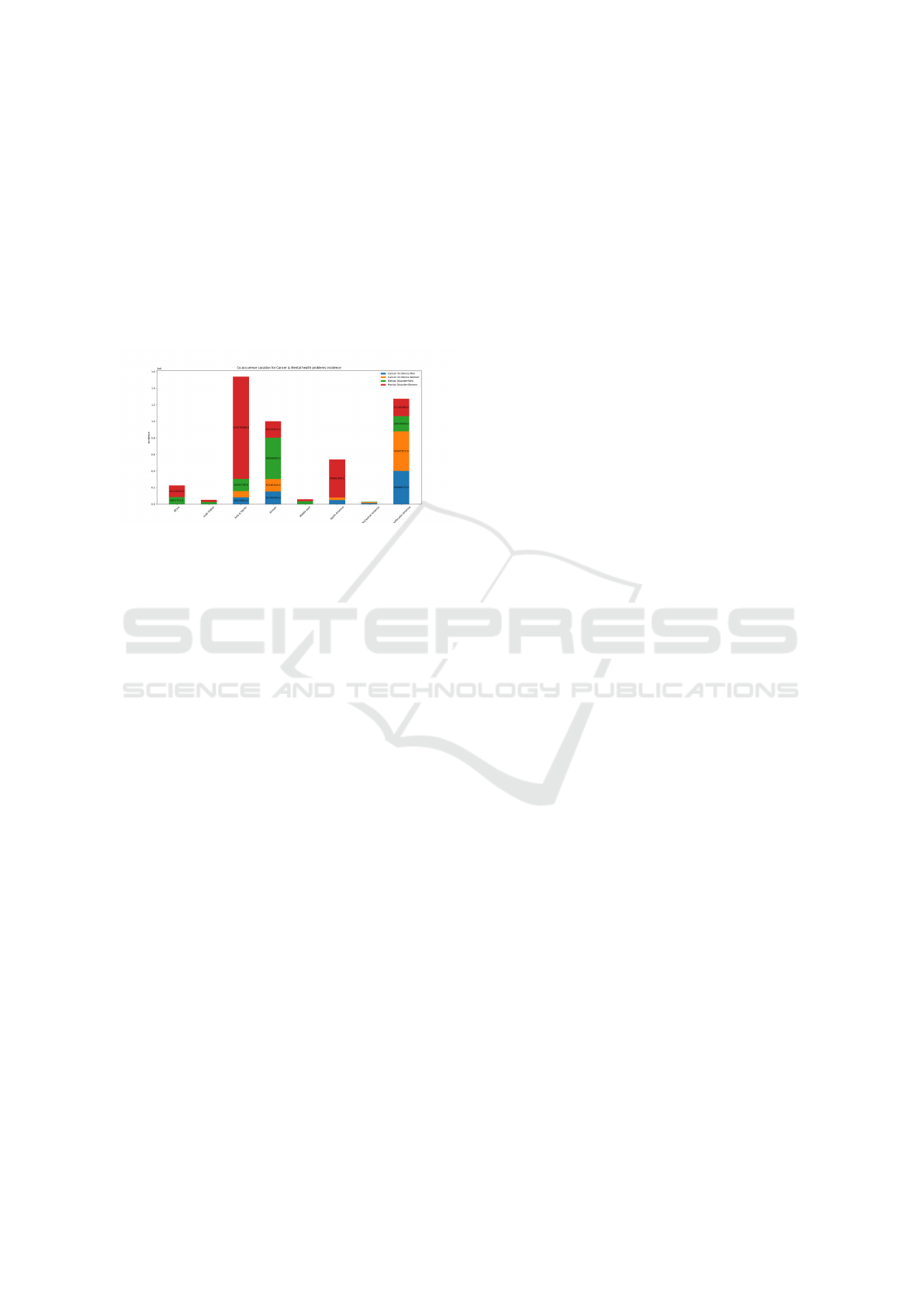
On the other hand, Figure 22 shows the location co-
occurrence analysis over our experimental setup. It
should be noted that a higher number of cancer and
mental disorders were still registered in Asia & Pa-
cific and Europe regions, while Africa had low num-
bers of incidence of the considered health diseases.
6 CONCLUSIONS AND FUTURE
WORK
This paper has presented and experimentally assessed
Drill-CODA, a framework designed for supporting
drill-across multidimensional big data analytics on
Privacy-Preserving Big Hierarchical Data Analytics via Co-Occurrence Analysis
101

large-scale co-occurrence aggregate hierarchical data.
Future work is mainly oriented towards extend-
ing our proposed framework by means of innova-
tive characteristics of the emerging big data process-
ing paradigm, such as: (i) management of uncertain
and imprecise hierarchical data (e.g., (Burdick et al.,
2007)); (ii) anomaly detection (e.g., (Langone et al.,
2020)); (iii) inference detection (e.g., (Chow et al.,
2008)); (iv) explainability (e.g., (Aghaeipoor et al.,
2022)); (v) visualization (e.g., (Cuzzocrea and Mans-
mann, 2009; Barkwell et al., 2018)).
Figure 22: Location Co-Occurrence Analysis over the
Cancer-Incidence/Mental-Disorders Experimental Setup.
ACKNOWLEDGEMENTS
This work was funded by the Next Generation EU
- Italian NRRP, Mission 4, Component 2, Invest-
ment 1.5 (Directorial Decree n. 2021/3277) - project
Tech4You n. ECS0000009.
REFERENCES
Aghaeipoor, F., Javidi, M. M., and Fern
´
andez, A. (2022).
IFC-BD: an interpretable fuzzy classifier for boosting
explainable artificial intelligence in big data. IEEE
Trans. Fuzzy Syst., 30(3):830–840.
Agrawal, R., Srikant, R., and Thomas, D. (2005). Privacy
preserving OLAP. In Proceedings of the ACM SIG-
MOD International Conference on Management of
Data, Baltimore, Maryland, USA, June 14-16, 2005,
pages 251–262. ACM.
Barkwell, K. E., Cuzzocrea, A., Leung, C. K., Ocran, A. A.,
Sanderson, J. M., Stewart, J. A., and Wodi, B. H.
(2018). Big data visualisation and visual analytics
for music data mining. In 22nd International Con-
ference Information Visualisation, IV 2018, Fisciano,
Italy, July 10-13, 2018, pages 235–240. IEEE Com-
puter Society.
Burdick, D., Deshpande, P. M., Jayram, T. S., and Al., E.
(2007). OLAP over uncertain and imprecise data.
VLDB J., 16(1):123–144.
Chow, R., Golle, P., and Staddon, J. (2008). Detecting pri-
vacy leaks using corpus-based association rules. In
Proceedings of the 14th ACM SIGKDD international
conference on Knowledge discovery and data mining,
pages 893–901.
Corder, G. W. and Foreman, D. I. (2014). Nonparametric
Statistics: A Step-by-Step Approach. Wiley.
Cuzzocrea, A. (2023). A reference architecture for support-
ing multidimensional big data analytics over big web
knowledge bases: Definitions, implementation, case
studies. Int. J. Semantic Comput., 17(4):545–568.
Cuzzocrea, A., Furfaro, F., Greco, S., Masciari, E., Mazzeo,
G. M., and Sacc
`
a, D. (2005). A distributed sys-
tem for answering range queries on sensor network
data. In 3rd IEEE Conference on Pervasive Comput-
ing and Communications Workshops (PerCom 2005
Workshops), 8-12 March 2005, Kauai Island, HI,
USA, pages 369–373. IEEE Computer Society.
Cuzzocrea, A., Furfaro, F., and Sacc
`
a, D. (2003). Hand-
olap: A system for delivering OLAP services on hand-
held devices. In 6th International Symposium on Au-
tonomous Decentralized Systems (ISADS 2003), 9-11
April 2003, Pisa, Italy, pages 80–87. IEEE Computer
Society.
Cuzzocrea, A. and Mansmann, S. (2009). OLAP visualiza-
tion: models, issues, and techniques. In Encyclopedia
of Data Warehousing and Mining, Second Edition (4
Volumes), pages 1439–1446. IGI Global.
Devastator, T. (2023). Mental health disorder.
Honda, K., Oda, T., Tanaka, D., and Notsu, A. (2015).
A collaborative framework for privacy preserving
fuzzy co-clustering of vertically distributed cooccur-
rence matrices. Advances in Fuzzy Systems, 2015:art.
729072.
Langone, R., Cuzzocrea, A., and Skantzos, N. (2020). In-
terpretable anomaly prediction: Predicting anomalous
behavior in industry 4.0 settings via regularized logis-
tic regression tools. Data Knowl. Eng., 130:101850.
Organization, W. H. (2023). Cancer incidence.
Ouazzani, Z. E., Braeken, A., and Bakkali, H. E. (2021).
Proximity measurement for hierarchical categorical
attributes in big data. Secur. Commun. Networks,
2021:6612923:1–6612923:17.
Ram Mohan Rao, P., Murali Krishna, S., and Siva Kumar,
A. (2018). Privacy preservation techniques in big data
analytics: a survey. Journal of Big Data, 5(1):33.
Russom, P. (2011). Big data analytics. TDWI Best Practices
report, Fourth Quarter, 19(4):1–34.
Singh, A. K. and Kumar, J. (2023). A privacy-preserving
multidimensional data aggregation scheme with se-
cure query processing for smart grid. J. Supercomput.,
79(4):3750–3770.
Tran, H.-Y. and Hu, J. (2019). Privacy-preserving big data
analytics a comprehensive survey. Journal of Parallel
and Distributed Computing, 134:207–218.
Tsai, C.-W., Lai, C.-F., Chao, H.-C., and Vasilakos, A. V.
(2015). Big data analytics: a survey. Journal of Big
data, 2:1–32.
Wang, J., Fang, S., Liu, C., Qin, J., Li, X., and Shi, Z.
(2020). Top-k closed co-occurrence patterns mining
with differential privacy over multiple streams. Fu-
ture Gener. Comput. Syst., 111:339–351.
DATA 2024 - 13th International Conference on Data Science, Technology and Applications
102

Wang, S., Sinnott, R., and Nepal, S. (2018). Pairs: Privacy-
aware identification and recommendation of spatio-
friends. In 2018 17th IEEE International Confer-
ence On Trust, Security And Privacy In Computing
And Communications/12th IEEE International Con-
ference On Big Data Science And Engineering (Trust-
Com/BigDataSE), pages 920–931.
Wei, Y., Jia, J., Wu, Y., Hu, C., Dong, C., Liu, Z., Chen, X.,
Peng, Y., and Wang, S. (2024). Distributed differen-
tial privacy via shuffling versus aggregation: A curi-
ous study. IEEE Trans. Inf. Forensics Secur., 19:2501–
2516.
Wu, Y., Weng, D., Deng, Z., Bao, J., Xu, M., Wang, Z.,
Zheng, Y., Ding, Z., and Chen, W. (2021). Towards
better detection and analysis of massive spatiotempo-
ral co-occurrence patterns. IEEE Trans. Intell. Transp.
Syst., 22(6):3387–3402.
Privacy-Preserving Big Hierarchical Data Analytics via Co-Occurrence Analysis
103