
CVE2CWE: Automated Mapping of Software Vulnerabilities to
Weaknesses Based on CVE Descriptions
Massimiliano Albanese
a
, Olutola Adebiyi
b
and Frank Onovae
c
Center for Secure Information Systems, George Mason University, Fairfax, U.S.A.
Keywords:
Vulnerabilities, Vulnerability Classification, Security Metrics, Software Weaknesses.
Abstract:
Vulnerabilities in software systems are inevitable, but proper mitigation strategies can greatly reduce the risk to
organizations. The Common Vulnerabilities and Exposures (CVE) list makes vulnerability information read-
ily available and organizations rely on this information to effectively mitigate vulnerabilities in their systems.
CVEs are classified into Common Weakness Enumeration (CWE) categories based on their underlying weak-
nesses and semantics. This classification provides an understanding of software flaws, their potential impacts,
and means to detect, fix and prevent them. This understanding can help security administrators efficiently
allocate resources to address critical security issues. However, mapping of CVEs to CWEs is mostly a manual
process. To address this limitation, we introduce CVE2CWE, an automated approach for mapping Common
Vulnerabilities and Exposures (CVEs) to Common Weakness Enumeration (CWE) entries. Leveraging natural
language processing techniques, CVE2CWE extracts relevant information from CVE descriptions and maps
them to corresponding CWEs. The proposed method utilizes TF-IDF vector representations to model CWEs
and CVEs and assess the semantic similarity between CWEs and previously unseen CVEs, facilitating accu-
rate and efficient mapping. Experimental results demonstrate the effectiveness of CVE2CWE in automating
the vulnerability-to-weakness mapping process, thereby aiding cybersecurity professionals in prioritizing and
addressing software vulnerabilities more effectively. Additionally, we study the similarities and overlaps be-
tween CWEs and quantitatively assess their impact on the classification process.
1 INTRODUCTION
A vulnerability is a flaw or defect, commonly found
in software or hardware, which has the potential to be
exploited by attackers for malicious purposes. On the
other hand, a software weakness represents a group
or category of vulnerabilities that share similar char-
acteristics or traits. The Common Vulnerabilities and
Exposures (CVE) system was introduced to provide
a unified method for publicly disclosing security vul-
nerabilities, and it is referenced as a standard in the
cybersecurity world. The Common Weakness Enu-
meration (CWE) is a catalog of software and hard-
ware weakness types that serves as a foundational
resource for identifying, mitigating, and preventing
weaknesses. CWE serves as a comprehensive list
of software vulnerabilities, with a focus on founda-
tional errors. In contrast, CVE encompasses doc-
umented instances of vulnerabilities associated with
a
https://orcid.org/0000-0002-3207-5810
b
https://orcid.org/0000-0002-2675-5096
c
https://orcid.org/0009-0008-7504-8179
specific systems or products. The purpose of classi-
fying CVEs into CWE is to provide an easy way to
identify specific types of weaknesses and also under-
stand the nature of vulnerabilities. CWE facilitates
the identification and recognition of specific types of
vulnerabilities and enables deeper analysis of the root
causes and common patterns associated with specific
weaknesses. This understanding is important for se-
curity administrators to develop effective mitigation
and prevention strategies.
The volume of publicly disclosed vulnerabilities is
increasing and thousands of them are yet to be classi-
fied under a CWE category. CWE provides a valuable
vulnerability taxonomy for CVE entries, organized in
a hierarchical structure that allows for multiple lev-
els of abstraction of behaviors. The National Insti-
tute of Standards and Technology (NIST) oversees the
National Vulnerability Databases (NVD), which per-
forms analyses on CVE entries published in the CVE
list maintained by MITRE. The descriptions of CVEs
are manually analyzed and classified into CWE cat-
egories, but manual classification introduces delays
500
Albanese, M., Adebiyi, O. and Onovae, F.
CVE2CWE: Automated Mapping of Software Vulnerabilities to Weaknesses Based on CVE Descriptions.
DOI: 10.5220/0012770400003767
Paper published under CC license (CC BY-NC-ND 4.0)
In Proceedings of the 21st International Conference on Security and Cryptography (SECRYPT 2024), pages 500-507
ISBN: 978-989-758-709-2; ISSN: 2184-7711
Proceedings Copyright © 2024 by SCITEPRESS – Science and Technology Publications, Lda.

and errors. A recent approach to vulnerability clas-
sification adopted a transformer encoder-decoder ar-
chitecture and utilized a pure self-attention mecha-
nism (Wang et al., 2021).
In this study, we argue that CVE descriptions are
critical for appropriately classifying vulnerabilities.
Leveraging widely adopted Natural Language Pro-
cessing (NLP) principles, we present a methodology
for identifying distinguishing features of each CWE
category and mapping previously unseen CVEs to the
most likely CWE category. Furthermore, we study
the inherent similarities between CWEs, and quan-
tify the impact of such similarities on the overall clas-
sification accuracy of our approach. Our evaluation
demonstrates that our approach is effective in accu-
rately predicting the CWE category of a previously
unseen CVE based on its textual description.
The remainder of this paper is organized as fol-
lows. Section 2 discusses related work and Section 3
provides an overview of NLP concepts used in our
work. Next, Section 4 describes our approach to map-
ping CVEs to CWEs. Then Section 5 reports on our
evaluation of the approach and analysis of the results.
Finally, Section 6 gives some concluding remarks.
2 RELATED WORK
Various organizations, including MITRE and NIST,
attempt to classify vulnerabilities based on their un-
derlying weaknesses. As of August 2023, 212,700
vulnerabilities were published in NVD. Of these vul-
nerabilities, 158,873 had been classified under a CWE
category, leaving 53,827 with no CWE category as-
signed. CVEs tagged as “NVD-CWE-noinfo” sug-
gest that there is insufficient information to map them
to specific CWE categories, while those tagged as
“NVD-CWE-Other” do not easily fit into one of the
specific CWE categories. In both cases, the CVE de-
scriptions lack detailed information about the specific
weakness associated with the vulnerabilities, making
it difficult to manually classify them. MITRE classi-
fies vulnerabilities into Common Weakness Enumera-
tions (CWEs) for the purpose of providing a common
language for identifying, describing, and categorizing
security weaknesses. The categorization of vulnera-
bilities based on their security weaknesses can pro-
vide information to organizations to help in assessing
and prioritizing vulnerabilities based on their impact,
likelihood, and available mitigation strategies.
As CWEs are organized in a hierarchical struc-
ture, understanding the nature of weaknesses at var-
ious levels is significantly influenced by this struc-
ture. Categories positioned higher in the hierarchy
(e.g., Configuration) offer a comprehensive overview
of a vulnerability type and may have numerous as-
sociated child CWEs. In contrast, those positioned
at lower levels (e.g., Cross-Site Scripting) provide a
more detailed perspective at a finer level of granu-
larity, typically having fewer or no associated child
CWEs. MITRE has designed four hierarchy entry
types to provide clarity and understanding of the re-
lationships between weaknesses: Pillar, Class, Base,
and Variant. Pillars are top-level entries in the Re-
search Concepts View (CWE-1000), typically repre-
senting a type of weakness that describes a flaw. A
class is a more specific weakness that describes an
issue in terms of one or two dimensions: behavior,
property, and resource. A base weakness provides
sufficient details to infer a specific method for detec-
tion and prevention, typically describing two or three
dimensions. A variant usually involves a specific lan-
guage or technology, describing issues in terms of
three to five dimensions.
ThreatZoom (Aghaei et al., 2020) uses a mix of
text mining techniques and neural networks to auto-
matically map CVEs to CWEs. VrT (Alshaya et al.,
2020) uses machine learning (ML) to analyze vulner-
ability descriptions to map them to CWEs, but it was
only tested on the top 25 CWEs. Other studies have
proposed alternative approaches for classifying vul-
nerabilities (Chen et al., 2020; Davari et al., 2017; Pan
et al., 2023). By contrast, our work relies on simple
but effective NLP concepts rather than overly com-
plex ML solutions, resulting in an effective and effi-
cient solution of practical applicability. Furthermore,
we study the similarities between CWEs and evaluate
their impact on classification accuracy.
3 TECHNICAL BACKGROUND
The approach to analyzing vulnerabilities that we
present in this paper relies on data from the National
Vulnerability Database (NVD) and MITRE, and Nat-
ural Language Processing concepts including Term
Frequency - Inverse Document Frequency (TF-IDF)
and Cosine Similarity to determine the similarity level
between CVEs and CWEs.
3.1 TF-IDF Analysis
Term Frequency-Inverse Document Frequency (TF-
IDF) is a statistical measure widely used in natural
language processing and information retrieval to eval-
uate the importance of a word (or term) within a docu-
ment relative to a collection of documents (corpus). It
is based on the premise that the importance of a term
CVE2CWE: Automated Mapping of Software Vulnerabilities to Weaknesses Based on CVE Descriptions
501

to a document increases with its frequency within the
document (Term Frequency), and it is adjusted by
how rare the term is across the entire corpus (Inverse
Document Frequency). The Term Frequency (TF) of
a term t with respect to a document d is the frequency
of term t within document d, and it is calculated as
the number of times the term occurs in the document
divided by the total number of terms in the document.
TF(t, d) =
No. of times term t appears in doc d
Total no. of terms in doc d
(1)
The Inverse Document Frequency (IDF) of a term
t with respect to a document corpus D measures the
rarity of the term across the entire document corpus.
It is calculated as the logarithm of the total number
of documents divided by the number of documents
containing the term. A constant 1 is normally added
to the denominator of the argument of the log function
in the IDF formula in order to account for the presence
of terms that may not appear in any of the documents
in the corpus and prevent potential division by zero
errors. If a term occurs in all the documents in the
corpus, the argument of the log function is close to 1,
resulting in IDF being close to 0.
IDF(t, D) = log
|D|
1 + |{d ∈ D | t ∈ d}|
(2)
The TF-IDF score for a term t in a document d ∈ D
is computed by multiplying its TF by its IDF.
TF-IDF(t, d, D) = TF(t, d) · IDF(t, D) (3)
The Inverse Document Frequency reduces the
weight of terms that occur frequently across the en-
tire corpus, thus emphasizing terms that are unique or
specific to certain documents. As a result, terms with
high TF-IDF scores for a given document, are charac-
teristic of that particular document.
As described in detail in Section 4, the cor-
pus utilized in the study presented in this pa-
per comprises documents corresponding to Common
Weakness Enumeration (CWE) categories, with each
document constructed by merging the descriptions
of Common Vulnerabilities and Exposures (CVEs)
falling within that specific CWE category. The ob-
jective is to leverage the TF-IDF scores of terms oc-
curring in the description of CVEs to (i) predict the
CWE category of previously unseen CVEs; (ii) study
the similarity between CWEs to explain errors in the
classification of CVEs.
3.2 Cosine Similarity
Cosine similarity is a measure of similarity between
two vectors in an inner product space that measures
the cosine of the angle between them. It is widely
used in various fields such as information retrieval,
natural language processing, and machine learning to
quantify the similarity between documents or vectors
in a high-dimensional space. Given two vectors A and
B, their cosine similarity is defined by Eq. 4
cosine-similarity(A,B) =
A · B
∥A∥∥B∥
(4)
where · denotes the dot product of the two vec-
tors, and ∥A∥ and ∥B∥ denote the Euclidean norms
(lengths) of vectors A and B respectively. The cosine
similarity ranges from -1 to 1, with -1 indicating com-
plete dissimilarity (i.e., vectors pointing in opposite
directions), 0 indicating orthogonality (i.e., perpen-
dicular vectors), and 1 indicating complete similarity
(i.e., vectors pointing in the same direction).
Cosine similarity is often used to measure the sim-
ilarity between documents based on their TF-IDF vec-
tor representations – where each dimension represents
a term in the document corpus. Higher cosine similar-
ity indicates that the documents have similar content.
All the elements of TF-IDF vectors are equal to or
greater than 0, thus the smallest possible value of co-
sine similarity occurs when the vectors are orthogo-
nal. In this case, the dot product of the vectors is 0,
resulting in a cosine similarity of 0.
4 METHODOLOGY
In this section, we describe the proposed approach for
predicting the CWE label of a previously unseen CVE
based solely on its textual description. First, based on
the technical background discussed in Section 3, we
introduce some notations and key definitions.
4.1 Notations and Definitions
Let D = {CWE
i
} denote a document corpus, where
each document CWE
i
is the concatenation of the tex-
tual descriptions of all the CVEs in the corresponding
CWE category. Then let T denote the set of all unique
terms occurring within documents in D. The TF-IDF
vector of a document CWE
i
is defined as follows.
TF-IDF(CWE
i
)=
tf-idf
1
,. . . ,tf -idf
j
,. . . ,tf -idf
|T |
(5)
where tf -idf
j
= TF-IDF(t
j
,CWE
i
) is the TF-IDF score
of term t
j
∈ T for document CWE
i
. Having defined the
TF-IDF vector of a CWE
i
document, we can define the
similarity between two documents CWE
i
and CWE
j
as
the cosine similarity between their TF-IDF vectors.
sim
c
(CWE
i
,CWE
j
) =
TF-IDF(CWE
i
) · TF-IDF(CWE
j
)
∥TF-IDF(CWE
i
)∥∥TF-IDF(CWE
j
)∥
(6)
SECRYPT 2024 - 21st International Conference on Security and Cryptography
502

The similarity function defined by Eq. 6 serves
two purposes. First, we use it to assess the simi-
larity between the description of previously unseen
CVEs and known CWEs to identify their most likely
CWE category. Second, we leverage the similari-
ties between CWEs to explain some of the most fre-
quent classification errors in the mapping of CVEs to
CWEs. Figure 1 shows a heat map reporting the value
of the cosine similarity for any pair of CWEs, with
darker shades of green representing higher similarity.
The MITRE Research Concepts view organizes
weaknesses based on abstractions of their behavior
and is intended to facilitate research into weaknesses,
including their inter-dependencies. The hierarchical
view is illustrated in Figure 2, showing 7 top-level
CWEs (Pillars) under which the top 25 CWEs are or-
ganized. To provide an alternative measure of simi-
larity between CWEs, in addition to the metric based
on the cosine similarity between their TF-IDF repre-
sentations, we defined a metric based solely on the
relative position of CWEs within this hierarchy.
Let d
i
denote the depth within the CWE hierarchy
of CWE
i
, with the depth of top-level entries (referred
to as Pillars) being equal to 1. Given two CWEs CWE
i
and CWE
j
that are directly connected in a parent-child
relationship, we define their similarity as
sim
h
(CWE
i
,CWE
j
) =
min(d
i
,d
j
)
max(d
i
,d
j
)
(7)
The rationale for Eq. 7 is that, deeper into the hier-
archy, differences between CWEs become relatively
smaller. For instance, based on Eq. 7, the similarity
between a pillar CWE (at depth 1) and its children
(at depth 2) is 0.5, whereas the similarity between its
children and their children (at depth 3) is 0.67.
Given two arbitrary CWEs CWE
i
and CWE
j
un-
der the same pillar CWE, let P(CWE
i
,CWE
j
) =
⟨CWE
k
1
,. . . , CWE
k
n
⟩, with k
1
= i and k
n
= j, denote
the shortest path between CWE
i
and CWE
j
. Then, the
hierarchy-bases similarity between CWE
i
and CWE
j
can be defined as
sim
h
(CWE
i
,CWE
j
) =
∏
1≤l<n
min(d
k
l
,d
k
l+1
)
max(d
k
l
,d
k
l+1
)
(8)
If CWE
i
and CWE
j
are not under the same pillar
CWE, then sim
h
(CWE
i
,CWE
j
) = 0. Based on Eq. 8,
the similarity between children of the same pillar
CWE (at depth 1) is 0.25, whereas the similarity be-
tween children of a CWE at depth 2 is 0.44, consis-
tent with the intuition that differences between CWEs
deeper in the hierarchy are smaller.
4.2 Data Collection and Processing
The vulnerability data (CVEs) for each CWE cate-
gory used in our experiments was collected from the
National Vulnerability Database (NVD). Initially, we
focused on the Top 25 CWEs
1
, and subsequently ex-
panded the corpus with additional CWEs. The CVEs
within each CWE category were randomly split into
training and test sets, as illustrated in Figure 3. For the
purpose of our evaluation, we used testing set sizes of
10, 20, and 40 CVEs per CWE category, i.e., we ran-
domly selected 10 CVEs from each CWE category
and set them aside for testing. We then used all other
CVEs to build a document corpus to be used for train-
ing. This corpus comprises one document for each
CWE category, obtained by merging the textual de-
scriptions of all the CVEs in the training set. Next, we
repeated this process twice, by randomly selecting 20
and 40 CVEs respectively for each CWE category.
The training corpus was used to characterize each
CWE in terms of its TF-IDF vector. This allowed us
to identify the most distinctive terms for each class of
vulnerabilities, thus facilitating the subsequent classi-
fication of CVEs in the test set into CWEs categories.
To strike a balance between efficiency and the
need to adequately characterize each document in the
corpus, we only considered the terms with a TF-IDF
score exceeding a predefined threshold. While retain-
ing information about the most representative terms,
this approach enables us to increase the sparsity of
TF-IDF vectors, thus improving computational effi-
ciency and memory utilization. In our evaluation, we
used a threshold of 0.1. Figure 4 illustrates an ex-
ample of the results obtained using the data in the
training corpus for computing TD-IDF vectors for
each CWE document. In particular, Figure 4 shows
the most representative terms for the top 3 CWEs:
(1) CWE-787, Out-of-bounds Write; (2) CWE-79,
Improper Neutralization of Input During Web Page
Generation (’Cross-site Scripting’); and (3) CWE-89,
Improper Neutralization of Special Elements used in
an SQL Command (’SQL Injection’).
As this example illustrates, and our experimental
evaluation in Section 5 confirms, each CWE docu-
ment can be adequately characterized using the 10-15
most representative terms out of the 240,768 unique
terms found across the Top 25 CWEs.
In the testing phase, each CVE in the testing
dataset was provisionally added to the training corpus
as a document CVE
x
consisting solely of the textual
description of that CVE, so as to enable us to calcu-
late its TF-IDF representation with respect to that cor-
pus. Its TF-IDF vector was then compared with the
1
https://cwe.mitre.org/top25/
CVE2CWE: Automated Mapping of Software Vulnerabilities to Weaknesses Based on CVE Descriptions
503

CWE-787 CWE-79 CWE-89 CWE-416 CWE-78 CWE-20 CWE-125 CWE-22 CWE-352 CWE-434 CWE-862 CWE-476 CWE-287 CWE-190 CWE-502 CWE-77 CWE-119 CWE-798 CWE-918 CWE-306 CWE-362 CWE-269 CWE-94 CWE-863 CWE-276
CWE-787 1 0.250896 0.212393 0.594872 0.439826 0.577562 0.670208 0.314311 0.183594 0.399856 0.39844 0.278023 0.376738 0.537092 0.486306 0.399818 0.75794 0.28229 0.219009 0.394435 0.435149 0.484348 0.411496 0.437997 0.414856
CWE-79 0.250896 1 0.297151 0.243543 0.34327 0.393882 0.180098 0.325348 0.457914 0.336834 0.239569 0.119374 0.354687 0.142094 0.311994 0.299715 0.28917 0.2084 0.208771 0.299037 0.199059 0.301793 0.411908 0.328114 0.262204
CWE-89 0.212393 0.297151 1 0.207411 0.489808 0.362903 0.161311 0.350637 0.230174 0.356751 0.190256 0.108222 0.323505 0.131953 0.321959 0.466096 0.272676 0.178641 0.18281 0.255729 0.173889 0.245235 0.548636 0.251134 0.20202
CWE-416 0.594872 0.243543 0.207411 1 0.399796 0.536306 0.504902 0.303838 0.184658 0.373555 0.33589 0.270563 0.382865 0.309501 0.463112 0.348071 0.552422 0.287495 0.207629 0.35361 0.477709 0.44962 0.40035 0.421551 0.390256
CWE-78 0.439826 0.34327 0.489808 0.399796 1 0.605584 0.314115 0.423034 0.276129 0.455081 0.35123 0.204955 0.518746 0.24296 0.526614 0.856307 0.413836 0.393678 0.298762 0.527541 0.333973 0.542495 0.515487 0.532332 0.450339
CWE-20 0.577562 0.393882 0.362903 0.536306 0.605584 1 0.508176 0.50847 0.336626 0.510129 0.461717 0.449642 0.671434 0.37831 0.576229 0.524512 0.697846 0.407514 0.374945 0.586814 0.549943 0.6196 0.596621 0.62089 0.557991
CWE-125 0.670208 0.180098 0.161311 0.504902 0.314115 0.508176 1 0.309382 0.158654 0.299141 0.456348 0.29578 0.353549 0.354289 0.366282 0.293057 0.445151 0.253374 0.200102 0.366319 0.388226 0.408934 0.268274 0.432488 0.404756
CWE-22 0.314311 0.325348 0.350637 0.303838 0.423034 0.50847 0.309382 1 0.262781 0.521038 0.298189 0.173911 0.443355 0.193719 0.396511 0.364639 0.349604 0.269765 0.283209 0.390128 0.287651 0.404824 0.535907 0.409476 0.411408
CWE-352 0.183594 0.457914 0.230174 0.184658 0.276129 0.336626 0.158654 0.262781 1 0.26114 0.270959 0.114115 0.390582 0.117578 0.260698 0.238933 0.213041 0.208427 0.409833 0.333186 0.169278 0.274585 0.298717 0.325527 0.243539
CWE-434 0.399856 0.336834 0.356751 0.373555 0.455081 0.510129 0.299141 0.521038 0.26114 1 0.291614 0.186733 0.39897 0.223108 0.502169 0.391714 0.392307 0.263212 0.268469 0.384052 0.282102 0.404861 0.657601 0.393935 0.397209
CWE-862 0.39844 0.239569 0.190256 0.33589 0.35123 0.461717 0.456348 0.298189 0.270959 0.291614 1 0.19804 0.454678 0.244814 0.391584 0.323803 0.246056 0.333981 0.262971 0.479682 0.398022 0.592921 0.2374 0.654239 0.629793
CWE-476 0.278023 0.119374 0.108222 0.270563 0.204955 0.449642 0.29578 0.173911 0.114115 0.186733 0.19804 1 0.24847 0.220502 0.216524 0.193483 0.325237 0.162261 0.145769 0.235536 0.293805 0.243794 0.179886 0.245579 0.233518
CWE-287 0.376738 0.354687 0.323505 0.382865 0.518746 0.671434 0.353549 0.443355 0.390582 0.39897 0.454678 0.24847 1 0.247939 0.472042 0.458617 0.403261 0.53449 0.3681 0.80151 0.394152 0.6069 0.451241 0.719685 0.551822
CWE-190 0.537092 0.142094 0.131953 0.309501 0.24296 0.37831 0.354289 0.193719 0.117578 0.223108 0.244814 0.220502 0.247939 1 0.254438 0.218787 0.449003 0.153098 0.132898 0.221706 0.282128 0.27196 0.23481 0.261116 0.245807
CWE-502 0.486306 0.311994 0.321959 0.463112 0.526614 0.576229 0.366282 0.396511 0.260698 0.502169 0.391584 0.216524 0.472042 0.254438 1 0.465393 0.427029 0.342083 0.314271 0.487183 0.348808 0.488458 0.540661 0.51339 0.446323
CWE-77 0.399818 0.299715 0.466096 0.348071 0.856307 0.524512 0.293057 0.364639 0.238933 0.391714 0.323803 0.193483 0.458617 0.218787 0.465393 1 0.345802 0.345762 0.269275 0.470867 0.303029 0.49457 0.431183 0.486921 0.41484
CWE-119 0.75794 0.28917 0.272676 0.552422 0.413836 0.697846 0.445151 0.349604 0.213041 0.392307 0.246056 0.325237 0.403261 0.449003 0.427029 0.345802 1 0.226733 0.204999 0.317028 0.423213 0.388639 0.548275 0.326669 0.304153
CWE-798 0.28229 0.2084 0.178641 0.287495 0.393678 0.407514 0.253374 0.269765 0.208427 0.263212 0.333981 0.162261 0.53449 0.153098 0.342083 0.345762 0.226733 1 0.247293 0.555402 0.268394 0.478654 0.227654 0.529997 0.445243
CWE-918 0.219009 0.208771 0.18281 0.207629 0.298762 0.374945 0.200102 0.283209 0.409833 0.268469 0.262971 0.145769 0.3681 0.132898 0.314271 0.269275 0.204999 0.247293 1 0.363588 0.213665 0.329827 0.253887 0.391779 0.330082
CWE-306 0.394435 0.299037 0.255729 0.35361 0.527541 0.586814 0.366319 0.390128 0.333186 0.384052 0.479682 0.235536 0.80151 0.221706 0.487183 0.470867 0.317028 0.555402 0.363588 1 0.350277 0.611401 0.334894 0.727632 0.57314
CWE-362 0.435149 0.199059 0.173889 0.477709 0.333973 0.549943 0.388226 0.287651 0.169278 0.282102 0.398022 0.293805 0.394152 0.282128 0.348808 0.303029 0.423213 0.268394 0.213665 0.350277 1 0.520434 0.299264 0.447362 0.464716
CWE-269 0.484348 0.301793 0.245235 0.44962 0.542495 0.6196 0.408934 0.404824 0.274585 0.404861 0.592921 0.243794 0.6069 0.27196 0.488458 0.49457 0.388639 0.478654 0.329827 0.611401 0.520434 1 0.336237 0.799907 0.784702
CWE-94 0.411496 0.411908 0.548636 0.40035 0.515487 0.596621 0.268274 0.535907 0.298717 0.657601 0.2374 0.179886 0.451241 0.23481 0.540661 0.431183 0.548275 0.227654 0.253887 0.334894 0.299264 0.336237 1 0.324581 0.290388
CWE-863 0.437997 0.328114 0.251134 0.421551 0.532332 0.62089 0.432488 0.409476 0.325527 0.393935 0.654239 0.245579 0.719685 0.261116 0.51339 0.486921 0.326669 0.529997 0.391779 0.727632 0.447362 0.799907 0.324581 1 0.759826
CWE-276 0.414856 0.262204 0.20202 0.390256 0.450339 0.557991 0.404756 0.411408 0.243539 0.397209 0.629793 0.233518 0.551822 0.245807 0.446323 0.41484 0.304153 0.445243 0.330082 0.57314 0.464716 0.784702 0.290388 0.759826 1
Figure 1: Similarity between CWEs in the Top 25.
CWE-1000
Pillar:
CWE-664
Pillar:
CWE-284
Pillar:
CWE-707
Pillar:
CWE-693
Pillar:
CWE-682
Pillar:
CWE-710
Class:
CWE-362
Pillar:
CWE-691
Class:
CWE-476
Class:
CWE-345
Composite:
CWE-352
Base:
CWE-190
Class:
CWE-20
Class:
CWE-74
Class:
CWE-943
Class:
CWE-94
Class:
CWE-77
Class:
CWE-913
Class:
CWE-79
Class:
CWE-668
Class:
CWE-669
Base:
CWE-89
Class:
CWE-610
Class:
CWE-118
Base:
CWE- 434
Base: CWE-
94
Class:
CWE-732
Base:
CWE-78
Base: CWE-
502
Base:
CWE-22
Class:
CWE-285
Class:
CWE-269
Class:
CWE-119
Base:
CWE-787
Class:
CWE-287
Base: CWE-
306
Class:
CWE-863
Class:
CWE-862
Base:
CWE-825
Base:
CWE-125
Base:
CWE-798
Class:
CWE-1391
Class:
CWE-1390
Base:
CWE-276
Variant:
CWE-416
Class:
CWE-441
Base:
CWE-918
Figure 2: CWE hierarchy: MITRE Research Concept view.
Tra ining Co rpus
CWE-787
CWE-79
CWE-416
CWE-89
CCAA IAB Meeting Presentation – Confidential & Proprietary 11
Creating a Document Corpus for Processing
CWE-787 = {CVE-2021-28664, CVE-2009-2550, …}
Training SetTe st in g Se t
Te st i n g D at a se t
CVE-2021-
28664
CVE-2021-
25926
CVE-2021-
42258
CVE-2023-
32530
CVE-2021-28664
CVE-2009-2550
Figure 3: Document Corpus.
CCAA IAB Meeting Presentation – Confide ntial & Proprietary 12
Training
Tra ining Corpus
CWE-787
CWE-79
CWE-416
CWE-89
term
TF
-IDF
overflow
0.32915214
buffer
0.27493886
code
0.25896131
cve
0.24692769
bounds
0.23922139
heap
0.19425047
memory
0.18389161
execution
0.1725813
write
0.16072639
arbitrary
0.15715205
attacker
0.15447129
user
0.15274369
crafted
0.13379966
stack
0.13040403
corruption
0.12767394
CWE-787
term
TF
-IDF
xss
0.47273918
scripting
0.36456737
cross
0.33896893
site
0.32069072
web
0.21963135
arbitrary
0.19596522
html
0.17719434
allows
0.17491908
remote
0.16700739
script
0.16142266
inject
0.15800978
attackers
0.1483744
php
0.13360246
parameter
0.12034736
CWE-79
term
TF
-IDF
sql
0.64277557
injection
0.38513733
php
0.28821384
parameter
0.24715491
remote
0.19953266
arbitrary
0.19220616
execute
0.19094692
commands
0.18209406
allows
0.17969005
attackers
0.16850951
CWE-89
Figure 4: Training.
TF-IDF vector of each CWE document in the corpus,
using the cosine similarity metric defined by Eq. 6, to
obtain a ranked list of CWE labels. Figure 5 shows a
generic CVE being added to the corpus and compared
against the CWE documents in the corpus.
Let T denote the testing set and let ℓ(CVE
x
) de-
note the correct CWE label for a CVE
x
∈ T . Then,
let ⟨ℓ
1
(CVE
x
), ℓ
2
(CVE
x
),. . . , ℓ
k
(CVE
x
)⟩ denote an or-
dered sequence of the top k labels ranked based on the
similarity sim
c
(CVE
x
,CWE
j
) between CVE
x
and the
corresponding CWE documents. The label ℓ
1
(CVE
x
)
identifies the most likely CWE that CVE
x
should be
assigned to according to our classification approach.
3
term
TF
-IDF
overflow
0.32915214
buffer
0.27493886
code
0.25896131
….
…
CWE-787
term
TF
-IDF
xss
0.47273918
scripting
0.36456737
cross
0.33896893
…
…
CWE-79
term
TF
-IDF
sql
0.64277557
injection
0.38513733
php
0.28821384
…
..
CWE-89
term
TF
-IDF
term
-1
0.32915214
term
-2
0.27493886
term
-3
0.25896131
….
…
CVE-X
Tra ining Corpus
CWE-787
CWE-79
CWE-416
CWE-89
CVE-X
Figure 5: Testing.
To assess the quality of the predicted CWE labels,
we define P
1
as the subset of test CVEs that are cor-
rectly mapped to their true label, i.e., CVE
x
∈ P
1
if the
highest ranking label ℓ
1
(CVE
x
) is equal to the true la-
bel ℓ(CVE
x
).
P
1
=
{
CVE
x
∈ T |ℓ
1
(CVE
x
) = ℓ(CVE
x
)
}
(9)
The definition of P
1
can be generalized to cap-
ture the subset of test CVEs such that their true label
ℓ(CVE
x
) is one the the top k ranked labels.
P
k
=
k
[
j=1
CVE
x
∈ T |ℓ
j
(CVE
x
) = ℓ(CVE
x
)
(10)
To study the performance of the proposed ap-
proach for individual CWEs, we can compute
P
k
(CWE
i
) as
P
k
(CWE
i
) = P
k
∩ T (CWE
i
) (11)
where T (CWE
i
) = {CVE
x
∈ T |ℓ(CVE
x
) = CWE
i
} is
the set of test CVEs from CWE
i
. Finally, we compute
the ratio ρ
k
of the number of CVEs with the correct la-
bel among the top k ranked labels to the total number
of test CVEs.
ρ
k
=
|P
k
|
|T |
(12)
Similarly to what we did for P
k
, we can evaluate
this ratio for individual CWEs.
ρ
k
(CWE
i
) =
|P
k
(CWE
i
)|
|T (CWE
i
)|
(13)
SECRYPT 2024 - 21st International Conference on Security and Cryptography
504
In our evaluation, we will focus on assessing P
1
,
P
2
, and P
3
, thus we will report on the values of |P
1
|,
|P
2
|, |P
3
|, ρ
1
, ρ
2
, and ρ
3
.
Table 1: CWE label prediction results for the Top 25 CWEs.
CWE ID |
|
|T |
|
| |
|
|P
P
P
1
1
1
|
|
| |
|
|P
P
P
2
2
2
|
|
| |
|
|P
P
P
3
3
3
|
|
| ρ
ρ
ρ
1
1
1
ρ
ρ
ρ
2
2
2
ρ
ρ
ρ
3
3
3
1 CWE-787 40 23 30 38 57.50% 75.00% 95.00%
2 CWE-79 40 36 38 38 90.00% 95.00% 95.00%
3 CWE-89 40 39 39 39 97.50% 97.50% 97.50%
4 CWE-416 40 33 38 39 82.50% 95.00% 97.50%
5 CWE-78 40 24 36 37 60.00% 90.00% 92.50%
6 CWE-20 40 18 26 30 45.00% 65.00% 75.00%
7 CWE-125 40 30 35 36 75.00% 87.50% 90.00%
8 CWE-22 40 31 34 36 77.50% 85.00% 90.00%
9 CWE-352 40 37 39 39 92.50% 97.50% 97.50%
10 CWE-434 40 28 34 34 70.00% 85.00% 85.00%
11 CWE-862 40 26 26 27 65.00% 65.00% 67.50%
12 CWE-476 40 34 34 36 85.00% 85.00% 90.00%
13 CWE-287 40 22 29 31 55.00% 72.50% 77.50%
14 CWE-190 40 29 34 34 72.50% 85.00% 85.00%
15 CWE-502 40 28 36 36 70.00% 90.00% 90.00%
16 CWE-77 40 24 30 31 60.00% 75.00% 77.50%
17 CWE-119 40 25 32 36 62.50% 80.00% 90.00%
18 CWE-798 40 33 35 36 82.50% 87.50% 90.00%
19 CWE-918 40 39 39 40 97.50% 97.50% 100.00%
20 CWE-306 40 16 27 31 40.00% 67.50% 77.50%
21 CWE-362 40 28 30 32 70.00% 75.00% 80.00%
22 CWE-269 40 25 34 37 62.50% 85.00% 92.50%
23 CWE-94 40 30 33 35 75.00% 82.50% 87.50%
24 CWE-863 40 20 29 32 50.00% 72.50% 80.00%
25 CWE-276 40 21 28 35 52.50% 70.00% 87.50%
Total 1,000 699 825 875 69.90% 82.50% 87.50%
5 EXPERIMENTAL EVALUATION
In this section, we report the results of our experimen-
tal evaluation of the proposed approach for predicting
the classification of previously unseen CVEs. First, in
Section 5.1, we present the results on a dataset com-
prising the top 25 CWEs. Then, in Section 5.2, we
extended the analysis to the top 50 CWEs.
5.1 Analysis for the Top 25 CWEs
Table 1 reports the results obtained using 40 CVEs
from each CWE for testing. The table reports the val-
ues of |P
1
|, |P
2
|, |P
3
|, ρ
1
, ρ
2
, and ρ
3
for each CWE
as well as the aggregate statistics. These results indi-
cate that in 69.9% of the cases, the true CWE label
of a CVE was correctly identified as the top-ranking
label. In 82.5% of the cases, the true CWE label of
a CVE was one of the top 2 ranking labels, whereas,
in 87.5% of the cases, the true CWE label of a CVE
was one of the top 3 ranking labels. We repeated this
evaluation for test sizes of 10 and 20 CVEs per CWE
and observed no significant difference in the values of
ρ
1
, ρ
2
, and ρ
3
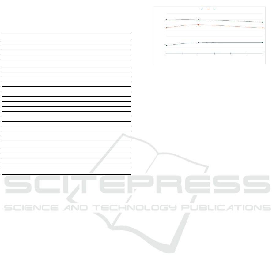
, as shown in Figure 6. This result is ex-
pected, as the training corpus is orders of magnitude
larger than the testing corpus, irrespective of whether
we set aside 10 or 20 CVEs per CWE for testing.
60%
65%
70%
75%
80%
85%
90%
95%
10 15 20 25 30 35 40
%
No. of test CVEs per CWE
⍴1 ⍴2 ⍴3
Figure 6: Accuracy vs. number of test CVEs per CWE.
Overall, these results indicate that several CVEs
belonging to one CWE category were misclassified
as members of another CWE category. In most of
these cases, however, the correct CWE label was as-
signed the second or third-best score, indicating that
our approach can provide reasonably accurate solu-
tions. Figure 7 shows a heat map indicating how many
test CVEs from each CWE category corresponding to
the rows were assigned to each of the CWE labels cor-
responding to the columns. Darker shades of green
indicate a higher number of CVEs from the CWE on
the row classified as members of the CWEs on the
columns. As expected, the darkest cells are on the di-
agonal, indicating that most CVEs are correctly clas-
sified. While most of the classification errors appear
to be randomly distributed, with most cells outside of
the diagonal indicating 0 classification errors, several
relatively darker cells can be noted outside of the di-
agonal. For instance, 12 CVEs from CWE-78 are mis-
classified as CWE-77. When comparing this heat map
with the heat map in Figure 1, we notice that CWE-78
and CWE-77 have a cosine similarity sim
c
of approx-
imately 86%, which intuitively explains why misclas-
sifications between these two CWEs are to be ex-
pected. Furthermore, the hierarchy in Figure 2 indi-
cates that CWE-77 and CWE-78 are in a parent-child
relationship, at a depth of 3 and 4 respectively, which
corresponds to a hierarchy-based similarity sim
h
of
75%. Consistently with these observations 9 CVEs
from CWE-77 are misclassified as CWE-78.
The observations discussed above can be gener-
alized to any pair of CWEs, forming the foundation
for defining adjusted accuracy metrics that consider
the inherent similarities and overlaps between CWEs.
The rationale is that the closer two CWE documents
CWE
i
and CWE
j
are, the more classification errors we
can anticipate. Consequently, the adjusted accuracy
scores should offset the effect of CWE similarities to
better capture the potential of the proposed approach.
Let C(CWE
i
,CWE
j
) denote the number of
CVEs in CWE category CWE
i
that are classi-
fied as members of CWE
j
, i.e., C(CWE
i
,CWE
j
) =
CVE2CWE: Automated Mapping of Software Vulnerabilities to Weaknesses Based on CVE Descriptions
505

CWE-787
CWE-79
CWE-89
CWE-416
CWE-78
CWE-20
CWE-125
CWE-22
CWE-352
CWE-434
CWE-862
CWE-476
CWE-287
CWE-190
CWE-502
CWE-77
CWE-119
CWE-798
CWE-918
CWE-306
CWE-362
CWE-269
CWE-94
CWE-863
CWE-276
CWE-787
23
0
0
1
1
3
2
0
0
1
2
0
0
1
0
0
5
0
1
0
0
0
0
0
0
CWE-79
0
36
0
0
0
0
0
0
1
0
0
0
0
0
0
0
1
0
0
0
0
0
1
1
0
CWE-89
0
0
39
0
1
0
0
0
0
0
0
0
0
0
0
0
0
0
0
0
0
0
0
0
0
CWE-416
0
0
0
33
0
2
0
0
0
0
1
0
0
0
0
0
2
0
0
1
1
0
0
0
0
CWE-78
0
0
0
0
24
0
0
0
0
1
0
0
0
0
0
12
0
1
0
0
0
0
2
0
0
CWE-20
0
0
0
0
2
18
0
0
0
3
3
1
2
0
2
1
2
0
1
2
0
1
2
0
0
CWE-125
2
0
0
1
0
4
30
0
0
0
0
0
0
1
0
0
1
0
0
0
0
1
0
0
0
CWE-22
0
0
0
0
0
0
0
31
0
4
0
0
0
0
1
0
0
0
0
0
0
1
1
2
0
CWE-352
0
0
0
0
1
0
0
0
37
0
0
0
0
0
0
0
1
0
0
0
0
0
0
1
0
CWE-434
0
0
0
0
0
2
0
0
0
28
0
0
0
0
1
0
0
0
0
0
0
0
7
2
0
CWE-862
0
0
0
0
1
1
1
0
0
1
26
0
0
0
0
0
0
0
0
0
0
1
1
8
0
CWE-476
1
0
0
0
0
2
0
1
0
0
1
34
0
0
0
0
0
0
0
0
1
0
0
0
0
CWE-287
0
0
0
0
0
4
0
0
0
1
1
0
22
0
0
0
0
1
2
2
0
1
3
2
1
CWE-190
3
0
0
0
0
2
0
0
0
0
2
0
0
29
0
0
4
0
0
0
0
0
0
0
0
CWE-502
0
0
0
0
3
1
0
0
0
1
0
0
0
0
28
1
0
0
0
0
0
0
3
3
0
CWE-77
0
0
0
0
9
1
0
0
0
1
0
0
0
0
3
24
0
0
0
0
0
1
1
0
0
CWE-119
4
0
0
1
0
2
2
0
0
1
0
2
0
2
0
0
25
0
0
0
0
0
1
0
0
CWE-798
0
0
0
0
0
1
0
0
0
1
1
0
1
0
1
0
0
33
0
1
0
0
0
1
0
CWE-918
0
0
0
0
0
0
0
0
0
0
0
0
0
0
1
0
0
0
39
0
0
0
0
0
0
CWE-306
0
0
0
0
0
3
0
0
0
2
0
0
11
0
0
0
0
0
1
16
1
0
0
6
0
CWE-362
1
0
0
2
0
3
0
1
0
1
0
0
1
0
0
0
0
0
0
0
28
0
0
3
0
CWE-269
0
0
0
0
0
1
0
0
0
0
2
0
1
0
0
0
4
1
0
0
0
25
0
2
4
CWE-94
0
0
0
0
3
2
0
0
0
0
0
0
0
0
2
0
1
0
0
0
0
1
30
0
1
CWE-863
0
0
0
0
0
2
0
0
0
2
2
0
1
0
2
1
0
1
1
1
0
4
1
20
2
CWE-276
0
0
0
0
2
0
0
0
0
1
8
0
1
0
0
0
0
0
0
0
1
1
0
5
21
Figure 7: CWE error heat map.
CVE
x
∈ CWE
i
| ℓ
1
(CVE
x
)=CWE
j
. Next, let
δ(CWE
i
) denote the number of vulnerabilities from
CWE category CWE
i
that are incorrectly classified.
δ(CWE
i
) =
∑
CWE
j
̸=CWE
i
C(CWE
i
,CWE
j
) (14)
Eq. 14 defines the number of classification er-
rors for CWE category CWE
i
. Next, let δ
e
(CWE
i
)
be the fraction of δ(CWE
i
) that can be explained by
considering the similarities between CWEs. We ar-
gue that each misclassification C(CWE
i
,CWE
j
), with
CWE
i
̸= CWE
j
, can be explained proportionally to the
similarity between CWE
i
and CWE
j
.
δ
e
(CWE
i
)=
∑
CWE
j
̸=CWE
i
sim(CWE
i
,CWE
j
) ·C(CWE
i
,CWE
j
)
(15)
where sim is any of the similarity functions defined
earlier. The residual error δ
r
(CWE
i
) = δ(CWE
i
) −
δ
e
(CWE
i
) is the fraction of δ(CWE
i
) that cannot be
explained by considering the similarities between
CWEs, thus it represents true classification errors. Fi-
nally we can define the adjusted |P
a
1
(CWE
i
)| metric as
|P
a
1
(CWE
i
)| = C(CWE
i
,CWE
i
) + δ
e
(CWE
i
) (16)
where C(CWE
i
,CWE
i
) = |P
1
(CWE
i
)|. The adjusted
metric ρ
a
1
can be defined as:
ρ
a
1
(CWE
i
) =
|P
a
1
(CWE
i
)|
|T (CWE
i
)|
(17)
We computed the adjusted metrics |P
a
1
| and ρ
a
1
for
the results presented in Table 1. The values of the ad-
justed metrics and the original metrics are reported
in Table 2, when using similarity function sim
c
in
Table 2: Adjusted accuracy metrics for Top 25 CWEs, when
using similarity function sim
c
in Eq. 15.
CWE ID |
|
|T |
|
| |
|
|P
P
P
1
1
1
|
|
| ρ
ρ
ρ
1
1
1
|
|
|P
P
P
a
a
a
1
1
1
|
|
| ρ
ρ
ρ
a
a
a
1
1
1
1 CWE-787 40 23 57.50% 32.85 82.13%
2 CWE-79 40 36 90.00% 37.49 93.72%
3 CWE-89 40 39 97.50% 39.49 98.72%
4 CWE-416 40 33 82.50% 36.34 90.86%
5 CWE-78 40 24 60.00% 36.16 90.39%
6 CWE-20 40 18 45.00% 30.35 75.88%
7 CWE-125 40 30 75.00% 35.09 87.72%
8 CWE-22 40 31 77.50% 35.24 88.10%
9 CWE-352 40 37 92.50% 37.81 94.54%
10 CWE-434 40 28 70.00% 34.91 87.28%
11 CWE-862 40 26 65.00% 33.63 84.06%
12 CWE-476 40 34 85.00% 35.84 89.61%
13 CWE-287 40 22 55.00% 32.36 80.91%
14 CWE-190 40 29 72.50% 33.65 84.13%
15 CWE-502 40 28 70.00% 34.29 85.71%
16 CWE-77 40 24 60.00% 34.94 87.36%
17 CWE-119 40 25 62.50% 33.36 83.40%
18 CWE-798 40 33 82.50% 35.97 89.92%
19 CWE-918 40 39 97.50% 39.31 98.29%
20 CWE-306 40 16 40.00% 32.42 81.06%
21 CWE-362 40 28 70.00% 33.35 83.37%
22 CWE-269 40 25 62.50% 34.18 85.46%
23 CWE-94 40 30 75.00% 35.00 87.49%
24 CWE-863 40 20 50.00% 32.26 80.66%
25 CWE-276 40 21 52.50% 32.94 82.34%
Total 1,000 699 69.90% 869.25 86.92%
Eq. 15, and in Table 3, when using similarity func-
tion sim
h
. As expected, the adjusted accuracy met-
rics have higher values than the corresponding origi-
nal metrics, and enable us to capture the true perfor-
mance of the proposed approach. We also notice that,
when using similarity function sim
h
, the values of the
adjusted metrics are lower than those achieved using
similarity function sim
c
, and that is also expected as
sim
h
is by definition more coarse-grained than sim
c
.
SECRYPT 2024 - 21st International Conference on Security and Cryptography
506

Table 3: Adjusted accuracy metrics for Top 25 CWEs, when
using similarity function sim
h
in Eq. 15.
CWE ID |
|
|T |
|
| |
|
|P
P
P
1
1
1
|
|
| ρ
ρ
ρ
1
1
1
|
|
|P
P
P
a
a
a
1
1
1
|
|
| ρ
ρ
ρ
a
a
a
1
1
1
1 CWE-787 40 23 57.50% 28.47 71.18%
2 CWE-79 40 36 90.00% 36.44 91.11%
3 CWE-89 40 39 97.50% 39.25 98.13%
4 CWE-416 40 33 82.50% 34.20 85.50%
5 CWE-78 40 24 60.00% 33.67 84.17%
6 CWE-20 40 18 45.00% 18.75 46.88%
7 CWE-125 40 30 75.00% 32.33 80.81%
8 CWE-22 40 31 77.50% 31.67 79.17%
9 CWE-352 40 37 92.50% 37.00 92.50%
10 CWE-434 40 28 70.00% 28.89 72.22%
11 CWE-862 40 26 65.00% 29.72 74.31%
12 CWE-476 40 34 85.00% 34.00 85.00%
13 CWE-287 40 22 55.00% 24.61 61.52%
14 CWE-190 40 29 72.50% 29.00 72.50%
15 CWE-502 40 28 70.00% 29.44 73.61%
16 CWE-77 40 24 60.00% 31.36 78.40%
17 CWE-119 40 25 62.50% 30.32 75.81%
18 CWE-798 40 33 82.50% 33.80 84.50%
19 CWE-918 40 39 97.50% 39.08 97.71%
20 CWE-306 40 16 40.00% 24.00 60.00%
21 CWE-362 40 28 70.00% 28.00 70.00%
22 CWE-269 40 25 62.50% 26.52 66.29%
23 CWE-94 40 30 75.00% 32.33 80.83%
24 CWE-863 40 20 50.00% 22.57 56.42%
25 CWE-276 40 21 52.50% 25.58 63.96%
Total 1,000 699 69.9% 761 76.1%
5.2 Analysis for the Top K CWEs
For the evaluation presented in the previous section,
we only considered CVEs in the Top 25 CWEs. In
the next set of experiments, we repeated our evalua-
tion for the Top k CWEs, with k between 10 and 50,
in increments of 5. Table 4 reports the results for the
aggregate values of |P
1
|, ρ
1
, |P
a
1
|, and ρ
a
1
. These re-
sults show that, as the number of CWE categories in-
creases, the classification accuracy decreases. How-
ever, this is expected due to increased complexity,
class imbalance, and reduced discriminative power.
Table 4: CWE label prediction results for the Top k CWEs.
k
k
k |
|
|T |
|
| |
|
|P
P
P
1
1
1
|
|
| ρ
ρ
ρ
1
1
1
|
|
|P
P
P
a
a
a
1
1
1
|
|
| ρ
ρ
ρ
a
a
a
1
1
1
10 400 342 85.50% 372.55 93.14%
15 600 486 81.00% 542.33 90.39%
20 800 605 75.63% 713.28 89.16%
25 1,000 699 69.90% 869.25 86.92%
30 1,200 810 67.50% 1,013.45 84.45%
35 1,400 914 65.29% 1161.62 82.97%
40 1,600 996 62.25% 1,310.98 81.94%
45 1,800 1084 60.22% 1,419.57 78.87%
50 2,000 1144 57.20% 1,518.10 75.90%
6 CONCLUSIONS
Classifying vulnerabilities into CWEs helps assess
the potential risks associated with different vulner-
abilities. This assessment aids security administra-
tors in prioritizing their efforts and effectively allo-
cating resources based on the prevalence of specific
CWEs. Our evaluation results indicate that accurately
describing a vulnerability is the initial step toward au-
tomatically and correctly classifying vulnerabilities
into a weakness category. The terms in a CVE de-
scription must uniquely describe that vulnerability to
distinguish it from CVEs in other CWEs. Our study
also reveals the impact of intrinsic CWE similarities
on the classification task. Future research will de-
velop guidelines for improving CVE descriptions and
CWE definitions, thus facilitating automation.
ACKNOWLEDGEMENTS
This work was partly funded by the National Science
Foundation (NSF) under award CNS-1822094.
REFERENCES
Aghaei, E., Shadid, W., and Al-Shaer, E. (2020). Threat-
Zoom: Hierarchical neural network for CVEs to
CWEs classification. In Proc. of the 16th EAI Intl.
Conf. on Security and Privacy in Communication Sys-
tems (SecureComm 2020), pages 23–41. Springer.
Alshaya, F. A., Alqahtani, S. S., and Alsamel, Y. A. (2020).
VrT: A CWE-based vulnerability report tagger: Ma-
chine learning driven cybersecurity tool for vulnera-
bility classification. In Proc. of the IEEE/ACM 1st
Intl. Workshop on Software Vulnerability (SVM 2020),
pages 23–41. IEEE.
Chen, J., Kudjo, P. K., Mensah, S., Brown, S. A., and Ako-
rfu, G. (2020). An automatic software vulnerability
classification framework using term frequency-inverse
gravity moment and feature selection. Journal of Sys-
tems and Software, 167.
Davari, M., Zulkernine, M., and Jaafar, F. (2017). An auto-
matic software vulnerability classification framework.
In Proc. of the 2017 Intl. Conf. on Software Security
and Assurance (ICSSA 2017), pages 44–49. IEEE.
Pan, M., Wu, P., Zou, Y., Ruan, C., and Zhang, T. (2023).
An automatic vulnerability classification framework
based on BiGRU-TextCNN. Procedia Computer Sci-
ence, 222:377–386.
Wang, T., Qin, S., and Chow, K. P. (2021). Towards vulnera-
bility types classification using pure self-attention: A
common weakness enumeration based approach. In
Proc. of the 24th IEEE Intl. Conf. on Computational
Science and Engineering (CSE 2021), pages 146–153.
IEEE.
CVE2CWE: Automated Mapping of Software Vulnerabilities to Weaknesses Based on CVE Descriptions
507
