Optimal Wireless Meter Deployment Using Evolutionary Algorithms

Siddhartha Shakya

, Kin Poon

, Ahmed Suliman

, Alia Aljasmi

, Huda Goian

and Ahoud Barzaiq

EBTIC, Khalifa University of Science and Technology, Abu Dhabi, U.A.E.

IoT & AI Operations, e&, Abu Dhabi, U.A.E.

Keywords: Wireless Meter Network Planning, Optimization, Genetic Algorithm, Estimation of Distribution Algorithm,

Simulated Annealing.

Abstract: Utility companies use smart wireless meters to automate the collection of meter readings. This requires them

to design and deploy a wireless meter network where each meter is connected to a central Data Concentrator

Unit (DCU), which is then connected to the control centre of the company. In this paper we investigate the

problem of wireless network meter deployment by means of evolutionary algorithms. We model the

deployment problem as an evolutionary optimization problem, explore two different encoding schemes for

the objective function, and test 4 different algorithms against 5 typical setups of the network in different areas.

Our results show that Simulated Annealing (SA) is the best performing algorithm for the tested instances of

the problem and has better reliability against the other compared algorithms The devised models and the

algorithm have been built into a tool that is being used in a real-world scenario.

1 INTRODUCTION

The supervision of resources such as water or

electricity is a challenge facing modern cities and

governments (Pimenta and Chaves, 2021). Such

resources are usually provisioned through a utility

company. In addition to providing resources, the

utility company is also responsible for billing

customers and predicting resource demand (Marais et

el., 2016). Facilitating these actions requires

companies to monitor and record customers’ usage.

Traditionally, this has been performed by deploying

mechanical meters that require visits from workers to

manually take readings (Pimenta and Chaves, 2021).

This process incurs additional costs, is time-

consuming and the possibility of human error is high.

To tackle these issues, utility companies have

begun shifting to wireless meters that allow

automated collection of readings (Marais et el.,

2016). Such meters mitigate the problems with

https://orcid.org/0000-0002-9924-9222

https://orcid.org/0009-0006-1762-7952

https://orcid.org/0000-0002-1962-0213

https://orcid.org/0009-0004-6588-2320

https://orcid.org/0009-0007-9117-7811

https://orcid.org/0009-0007-9814-8052

manual data collection. However, they present their

own set of challenges. It is not just about installing

the meters. Deploying infrastructure that supports a

Wireless Meter Network (WMN) and facilitates

automatic data collection from sensors and transfer to

a central database is also required. The core of such

networks consists of Data Concentrator Units (DCUs)

or Data Aggregation Points (DAPs) which are devices

responsible for communicating with smart sensors to

collect data and forward it to central data repository.

Placing the DCUs in optimal locations is of the

utmost importance because it greatly affects the

Quality of Service (QoS) of Wireless Meter Networks

(Kong, 2016). Therefore, it is necessary to place

DCUs in optimal locations to maximize the coverage

of the sensor network and be able to obtain readings

from all smart sensors, while reducing the cost by

minimizing the number of DCUs required.

In this paper, we focus on the optimal placement

of DCUs in scenarios where the locations of wireless

meters and feeders are known. A feeder location

332

Shakya, S., Poon, K., Suliman, A., Aljasmi, A., Goian, H. and Barzaiq, A.

Optimal Wireless Meter Deployment Using Evolutionary Algor ithms.

DOI: 10.5220/0012791900003758

Paper published under CC license (CC BY-NC-ND 4.0)

In Proceedings of the 14th International Conference on Simulation and Modeling Methodologies, Technologies and Applications (SIMULTECH 2024), pages 332-339

ISBN: 978-989-758-708-5; ISSN: 2184-2841

represents an existing location where electricity is

available, which is a preferred location to install a

DCU. A DCU is responsible for collecting the data

from one or more smart sensors. When a wireless

meter is assigned to a DCU, the minimum required

Received Signal Strength (RSS) must be fulfilled to

ensure that the DCU can receive an accurate reading

from the assigned wireless meter. If the RSS values

are not provided between a given wireless meter and

a feeder, a distance constraint can also be applied to

ensure that the wireless meter is within the covering

range. In addition, a DCU has a capacity constraint

which determines the maximum number of wireless

meters to be connected. Generally, there is a default

capacity for each DCU which can be varied according

to the requirements by the planners of the network.

The main contributions of the paper are as

follows:

1. Model the placement of DCUs as an optimization

problem and formulate an objective function

while satisfying the given constraints.

2. Implement different evolutionary algorithms for

optimizing DCU placement problem.

3. Present a comparison of the results obtained from

the implemented techniques.

The rest of the paper is structured as follows.

Section 2 presents the related work in the area.

Section 3 describes the problem formulation and

Section 4 demonstrates the proposed approach.

Section 5 presents the experimental results.

Conclusions and directions for future work are

discussed in Section 6.

2 RELATED WORKS

There have been various studies on the optimal

placement of DCUs with different requirements. In

(Gallardo et el., 2021) the authors tackle the DCU

placement problem by proposing a 2-step technique.

Firstly, the neighbourhoods in the problem are

divided into multiple sub-networks. Afterwards,

multiple clusters of DCUs with smart meters are

formed to minimize the distance between them. This

is achieved by using the K-Medoids algorithm. This

work has been applied to urban, suburban, and rural

areas to prove its validity.

In (Kong, 2016), the authors focus on assigning

wireless meters to DCUs in a wireless

Neighbourhood Area Network (NAN) to support a

certain required QoS level. The QoS is expressed in

terms of packet delay, packet error probability and

node outage probability. A model which is developed

based on those parameters predicts the number of

required DCUs and their locations. (Wang et al.,

2018) model the problem as a network partition

problem where the goal is to minimize the distance

between DCUs and wireless meters. A clustering-

based algorithm (CPDA) based on the Floyd Warshall

algorithm is proposed to partition the network and

identify ideal DCU locations.

In Tanakornpintong and Pirak (2021), the authors

propose a DCU placement optimization algorithm

that identifies the best DCU locations based on the

minimum hop count, average throughput, and delay.

This algorithm has been tested in urban, suburban,

and rural areas. Our approach is to explore various

encoding schemes and then apply different

evolutionary algorithms to solve the wireless meter

assignment problem.

3 THE PROPOSED APPROACH

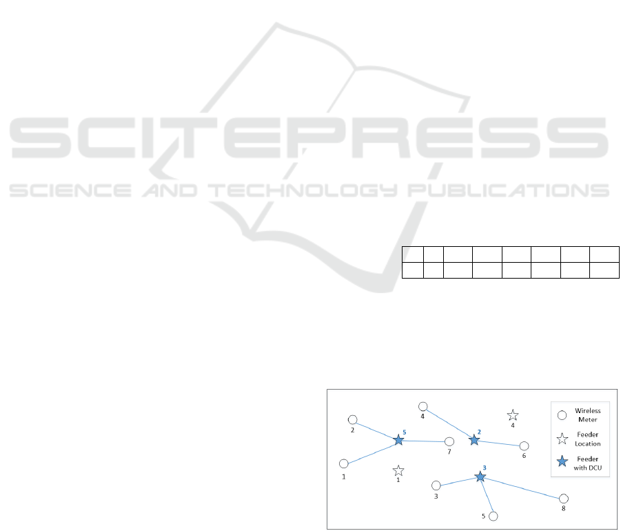
We investigate two possible encoding schemes to

assign each wireless meter to a DCU. The first one is

to model the solution as a string of integers, where the

length of the string is equal to the number of given

wireless meters. The individual value of the string is

equal to the index of the feeder to which should be

connected as shown below. Each meter is assigned to

one of the existing feeders which represent the

possible locations of DCUs. The feeder indices, that

do not appear in the solution string, are the ones not

being used.

feeder Index

meter Index

Figure 1 shows a network with the first encoding

scheme. In this example, there are 8 wireless meters

and 5 feeder locations, where feeder locations with

indices 2, 3 and 5 were chosen to be the DCU

locations.

Figure 1: Assignment of meters to DCUs using Encoding

Scheme 1.

Optimal Wireless Meter Deployment Using Evolutionary Algorithms

333

The advantage of this encoding lies in its

simplicity because the association between the meter

and DCU is explicitly presented in the given string.

The RSS or distance violation can be easily checked

by simply going through each value of the string with

its corresponding feeder. In Figure 1, meter 1 is

assigned to feeder 5. We can either obtain the RSS

value if it is provided in advance or calculate the

distance between these 2 nodes with their given

coordinates. However, there are two main drawbacks

of this encoding method. First, the size of the solution

space (i.e. the number of possible combinations) can

be very high. For the simple example given in Figure

1 with 8 meters and 5 feeders, the number of

combinations based on this encoding is equal to F^m

where F is the total number of feeders and m is the

total number of meters (i.e. 5^8= 390625 for above

example). The second disadvantage is that the chance

of obtaining a violated string after the genetic

operations (e.g. crossover and mutation in the case of

a Genetic Algorithm (Bäck et el, 1997) can also be

high. It is because this approach does not have any

control of the number of meters assigned to the

selected feeder. For example, after the crossover and

mutation operations, the generated string can be as

represented below:

feeder Index

meter Index

It indicates that 6 meters in total are assigned to

feeder 5 (where DCU will be installed), and 2 meters

to feeder 3. If each DCU can only accommodate 5

meters, feeder 5 will easily violate the capacity

constraint.

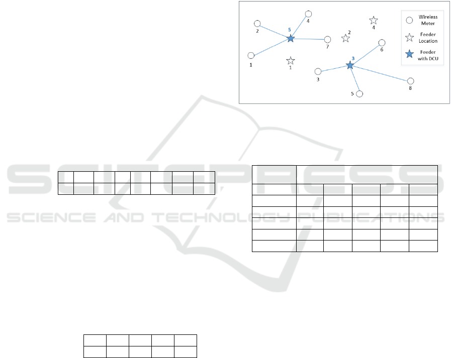
The second encoding scheme (see below) which

was adopted in this research is based on the binary

representation with a pre-calculated look-up table.

The selected feeders are 3 and 5 and the

corresponding connected network is depicted in

Figure 2.

Selected feeder

feeder Index

The assignment of meters to the selected DCUs is

purely based on the shortest distance (or the lowest

RSS). Therefore, meters 1, 2, 4 and 7 are assigned to

the selected feeder 5 whilst meters 3, 5, 6 and 8 are

assigned to feeder 3 as shown in Figure 2. This binary

encoding scheme has several advantages. First, the

number of combinations is significantly lower (i.e.

2^5 = 32 for the above example). The assignment of

meters is based on the shortest distance logic which

can implicitly create a nice cluster without the

possibility of any meter crossing another selected

cluster of DCU. The second advantage is that all the

standard n-point crossover and mutation based on the

binary encoding can be applied directly. However,

there is one drawback of this binary representation,

where the time required to calculate which meter

needs to be connected to which feeder can be high. It

is because it must run an assignment logic that in turn

requires a sorting logic to find the next nearest feeder

to a meter. However, this problem can be solved by

using a pre-calculated look up table as shown in Table

I with the given network in Figure 2.

Figure 2: Assignment of meters to DCUs using Encoding

Scheme 2.

Table 1: A lookup table for each feeder with its

corresponding meters.

Meter

Index

Neighbor feeder sorted according to

the given RSS or distances

The first column in the table stores all the meters

indices. The second column holds the first nearest

feeders to the corresponding meter as neighbouring

feeders in each row are sorted accordingly. We can

further speed up the RSS (or distance) comparison

between the feeder and the meter by limiting the

number of columns for the sorted feeders. For

example, only 3 feeders were considered for the first

meter as bolded in Table 1 based on the given

RSS/distance constraint. Each time when we need to

find the association between a feeder and a meter for

the selected DCU in the binary string, the look-up

table can be used to speed up the entire process,

especially when there are thousands of meters and

hundreds of feeders as in our case.

4 PROBLEM FORMULATION

Our problem can be formulated as below:

SIMULTECH 2024 - 14th International Conference on Simulation and Modeling Methodologies, Technologies and Applications

334

Sets

• M - A set of wireless meter locations.

• F - A set of feeders which are the possible

locations for DCUs.

• R – A matrix where 



represents the RSSI

between the 



meter and the 



feeder.

Decision Variable

• 



- Binary variable stating whether the 



feeder is being selected in GA string.

Deduced Variable Based on 



• 



– Binary variable stating whether the 



feeder is connected to the 



meter. The 



calculated based on the given look-up table and

the association between the selected feeder and

the nearest meters/RSS as discussed previously.

Parameters

• 



- Path distance connecting the



feeder and





meter

• 



- The unit cost to connect a feeder to a

meter.

• 



- The cost of a DCU being deployed.

• 





– Maximum allowable distance from the

feeder to a meter.

• 





– Maximum allowable RSS from the feeder

to a meter.

• - DCU capacity limit.

Minimize

  













 















(1)

  





 



  

(2)









 





     

(3)









 





     

(4)

The objective function (1) minimizes the cost of

connecting wireless meter to the selected DCU. This

cost is made of the link cost and DCU cost. If RSS is

used instead, the link cost can be set to 1, which is the

case for our purpose. Constraint (2) enforces the

capacity limit of DCUs. Either Constraint (3) or

Constraint 4 will be used depending on whether

distance or RSS is given at the first place.

5 EVOLUTIONARY

ALGORITHMS

The solution x = {x1, x2,.., xn} of an evolutionary

algorithm is a binary string where each x

represents

a feeder, i, and its value represents if the this feeder is

selected to be the location for the DCU (Eq 1). The

objective for the algorithm is to find a set of feeders

to be a DCU such that the objective function, f(x), as

defined in equation 1 is minimized. Four different

evolutionary algorithms have been implemented and

tested against this problem. They include two

univariate Estimation of distribution algorithms

(EDAs) (Larrañaga and Lozano, 2002) (Shakya and

Santana, 2012) (Pelikan and Goldberg, 2003),

Population Based Incremental Learning (PBIL)

(Baluja, 1994) and Distribution Estimation Using

Markov Network (DEUMd) (Shakya and McCall ,

2007, Shakya et el, 2018), a Genetic algorithm (GA)

(Goldberg, 1989), and a simulated annealing

algorithm (SA) (Kirkpatrick et. el, 1983). EDAs are a

class of evolutionary algorithms that model the

dependency between variables in a solution as a

probability distribution, estimate the parameters of

the probability distribution using the selected solution

and sample from the distribution to generate the new

population (Larrañaga and Lozano, 2002). This is

different to the crossover and mutation approach to

generating new population in a GA. The used EDAS

here are univariate EDA (Larrañaga and Lozano,

2002), where each variable, xi, in the solution x is

considered independent and a marginal probability

for each variable is calculated and sampled to

generate child population. Workflow from Univariate

EDAs are simpler in comparison to their bivariate or

multivariate counterparts. However, they have been

shown to work well on a wide range of optimization

problems (Larrañaga and Lozano, 2002, Shakya et. el,

2018, Bosman, 2003). The SA is one of the simplest

and effective EAs that is based on the concept of

Montecarlo Simulation (Kirkpatrick et. el, 1983). SA

has also been shown to work well on many real-world

optimization problems.

Workflow of each implemented algorithm is

described below.

1. Generate a population P consisting of M solutions

2. Build a breeding pool by selecting N promising

solutions from P using a selection strategy

3. Perform crossover on the breeding pool to generate

the population of new solutions

4. Perform mutation on the new solutions

5. Replace P with new solutions and go to step (2) until

the maximum number of generations (r) is reached

Optimal Wireless Meter Deployment Using Evolutionary Algorithms

335

PBIL

1. Initialize a probability vector p = {p

, p

, ..., p

} with

each p

= 0.5. Here, p

represents the probability of x

taking value 1 in the solution

2. Generate a population P consisting of M solutions by

sampling probabilities in p

3. Select set D from P consisting of N best solutions

4. Estimate probabilities of x

= 1 , for each x

, as









 

















5. Update each p

in p using p

= p

+ λ(p(x

= 1) − p

Here, 0 ≤ λ ≤ 1 is a parameter of the algorithm known

as the learning rate

6. Go to step 2 until the maximum number of

generations (r) is reached

DEUMd

1. Generate a population, P, consisting of M solutions

2. Select a set D from P consisting of N best solutions,

where N ≤ M.

3. For each solution, x, in D, build a linear equation

with the following form

η(F(x)) = α

+ α

+ ... + α

Where, function η(F(x)) < 0 is set to −ln(F(x)), for which

F(x), the fitness of the solution x, should be ≥ 1,

α = {α

+ α

+ ... + α

} are equation parameters, 0

values in binary variable x

are replaced with -1 for

creating linear equations.

4. Solve the build system of N equations to estimate α

5. Use α to estimate the distribution 























where









 







  















 







  





Here, β (inverse temperature coefficient) is set to β=g×

τ; g is the current iteration of the algorithm and τ is the

parameter known as the cooling rate.

6. Generate M new solution by sampling p(x) to

replace P and go to step 2 until the maximum number

of generations (r) is reached.

1. Randomly generate a solution x = {x

, x

, ..., x

}

2. For i = 1 to r do

a. Randomly mutate a variable in x to get x’

b. Set Δf = f(x’) − f(x)

c. Set x = x’ with probability













  





  

Where temperature coefficient T was set to T = 1/i×τ, i is

the current iteration, and τ is the parameter of the algorithm

called the cooling rate.

3. Terminate with answer x.

6 EXPERIMENTS AND RESULTS

In this paper, we used five different sample areas

from the data provided by our telecom partner for

testing the performance of the algorithms. These

areas represent a typical network size, in which our

partner is required to deploy smart meters with

different settings for feeders, meters and RSSI

distances. We denote them as Area1, Area2, Area3,

Area4 and Area5. The number of feeders were 408,

373, 519, 445 and 159, respectively for areas 1 to 5.

Similarly, the number of meters were 1826, 1275,

1485, 1133, 688 for areas 1 to 5 respectively. Also,

the maximum RSSI allowed (





) was set to -85

dbm, which meant any connection of a meter to

feeder with RSSI over -85 was counted as violation

and added to the link cost in equation 1. The value of

up to -85 was given the equal preference and therefore

had a 0 cost. The value for the total link cost, hence,

would be 0, if no link encoded in the solution is over

the RSSI limit of -85 dbm.

In addition, each algorithm has different set of

parameters that needs to be fine-tuned to obtain the

best results. We perform empirical analytics to find

the parameters for each algorithm where each

algorithm was run for 10 times with multiple settings

for each of the parameters, and those parameters that

provide the best average results were used as the

output of the algorithm.

Population size parameter (ps) for a population-

based algorithm such as GA, PBIL, and DEUMd,

ranged from 300 to 1000. The maximum generation

(mg) ranged from 500 to 1000. In addition, the elitism

(es) of 0 or 2 was used, i.e., either none or the best

two solutions from the previous generation were

copied to the next generation.

For the GA, four selection operators (so) were

tested, which included roulette wheel (rw),

tournament (tm), and two types of truncation

selection: one with selection size set to 0.5 of the

population size (tr0.5) and another with 0.3 (tr0.3)

(Bäck et el, 1997). The crossover operators (co) tested

were “simple one point” (op) and “uniform” (un)

crossovers with the probability of bit swapping set to

0.5 (un0.5). The mutation operator (mo) was set to

one-bit flip mutation (ob) [17]. In addition, the tested

crossover probabilities (cp) were 0.6 and 0.8, and the

mutation probabilities (mp) tested were 0.0001,

0.001, and 0.01, respectively.

For the PBIL, a truncation selection (Bäck et el,

1997) was used with 3 different settings for the size

of the selected population for recombination

operations (ss), which were 0.3, 0.5, 0.7 of the

population size. When the selection size is set to a

large value, the convergence of PBIL becomes slower

since the diversity is maintained for a longer period.

SIMULTECH 2024 - 14th International Conference on Simulation and Modeling Methodologies, Technologies and Applications

336

In addition, 5 different settings for learning rate

parameter (λ) were tested, 0.2, 0.1, 0.05, 0.01 and

0.005. Learning rate also controls the convergence of

the PBIL. The higher it is, the faster the population

converges and may not explore the search space

properly. Conversely, a lower learning rate means

better exploration at the expense of slower

convergence.

For the DEUMd, three different settings for

truncation selection were tested with selection size

(ss) set to 0.3, 0.5 and 0.7 of the population size. Also,

five different cooling rate settings (τ) were tested, 1,

0.5, 0.2, 0.1, and 0.05. Both selection size and the

cooling rate in DEUMd have a similar effect to the

selection size and learning rate in PBIL. They

determine the balance between exploration and

exploitation, leading to convergence of the algorithm.

For the SA, the maximum generation, r, was set

proportionally to other EAs population size and

maximum generation to ensure that the number of

fitness evaluations performed by all algorithms is the

same. In other words, the maximum generation for

the SA set to each combination of ps × mg used in

other population-based algorithms. The cooling rate

parameter in SA, which has a similar effect as the lr

and temperature coefficient in PBIL and DEUMd,

was tested against six different settings, 0.001,

0.0005, 0.0001, 0.00005, 0.00001 and 0.000005.

The results for the best set of parameters that

achieved the highest average fitness for each five

different areas are shown in Tables 2 to 5 for GA,

PBIL, DEUMd and SA respectively. The best values

for population size for GA (ps) was 1000 for all areas.

Hence, they are not shown in the table 2 to save space.

Table 2: Best performing parameters for GA.

Area

Area1

100

0.8

0.001

un0.5

Area2

500

0.8

0.001

un0.5

Area3

1000

0.8

0.001

un0.5

Area4

500

0.8

0.001

tr0.5

un0.5

Area5

1000

0.8

0.01

tr0.3

Table 3: Best performing parameters for PBIL.

Area

Area1

1000

300

0.1

Area2

1000

300

0.1

Area3

1000

300

0.1

Area4

1000

300

0.1

Area5

500

1000

150

0.2

Table 4: Best performing parameters for DEUMd.

Area

tau

Area1

300

1000

0.2

Area2

300

1000

0.5

Area3

300

1000

0.2

Area4

300

1000

0.2

Area5

300

1000

0.1

Table 5: Best performing parameters for SA.

Area

Area1

1000000

0.000005

Area2

1000000

0.000005

Area3

500000

0.00001

Area4

1000000

0.00001

Area5

500000

0.00001

Results in terms of mean fitness (AvgFit) together

with the standard deviation (SdFit) over the 10 runs

for each algorithm and for each of the 5 tested areas

is shown in Table 6. The minimum fitness (MnFit)

and maximum fitness (MxFit) found over the 10 runs

are also shown. The best performing values for each

area are highlighted in bold. We can notice that the

best performing algorithm in terms of the mean

fitness across all 5 area is SA, which is closely

followed by PBIL, the performance of GA and

DEUM is worse than that of the other two algorithms.

We can also notice that the standard deviation over

the 10 runs is lowest for SA in comparison to the other

tested algorithms, suggesting that the result for SA is

consistent and more predictable. For instance, for

Area1, the mean fitness of SA is 866 which is then

followed by 867 for PBIL, 869 for GA and 894 for

DEUMd. Similarly, the standard deviation for SA is

0.99, which is closely followed by 1.62 for PBIL,

1.57 by GA and 3.56 for DEUMd. Also, SA is better

in terms of Min and Max fitness with values of 865

and 868 respectively. The result pattern is similar

across the other 4 areas.

We also present result in terms of individual

objective values in Table 7 and Table 8, where Table

7 shows results in terms of best minimized RSSI for

each algorithm for each of the 5 tested areas, and

Table 8 shows the results in terms of the number of

clusters, i.e. the number of DCUs used for each

algorithm for each of the 5 tested areas. The lower the

RSSI values, the better the algorithm is and the lower

the DCU number used the better the solution is.

Similar to the results for the overall fitness, we show

the mean RSSI (AvgRS) together with the standard

deviation (SdRS) and also the minimum RSSI

(MnRS) and the minimum RSSI (MxRS), over the 10

runs of the algorithm for RSSI values. Similarly, we

show the mean number of DCU used (AvgDCU)

together with the standard deviation (SdDCU) and

also the minimum number of DCU used (MnDCU)

and the maximum number of DCU used (MxDCU),

over the 10 runs of the algorithm. Interestingly, all

algorithms were able to find the same RSSI sum

values across all areas (apart from area 5 and area 4

for some algorithms), over all the 10 runs, as seen on

Table 7. However, the number of DCU used is

different for different algorithms as seen on Table 8,

suggesting that this objective is the contributor for the

Optimal Wireless Meter Deployment Using Evolutionary Algorithms

337

overall fitness difference. Hence, we can notice that

the average number of DCU used by SA is best for

each of the 5 areas. Similarly lower standard

deviation of SA in comparison to other algorithms

suggests that it is the most predictable algorithm. The

design with lower number of DCU used is

particularly good as it results in less equipment, and

less energy consumption for the network, hence

reducing overall cost of the network.

Table 6: Fitness for each algorithm for each of the 5 tested

areas, where Maximum, Minimum and average together

with standard deviation of the fitness is shown for the 10

runs of each algorithm for each of the areas. Here, lower the

fitness the better the solution is.

Area

Algo

MnFit

MxFit

AvgFit

SdFit

Area1

866.2

871.2

869.7

1.57

Area1

PBIL

864.2

869.2

867.4

1.62

Area1

DEUM

892.2

904.2

894.9

3.56

Area1

865.2

868.2

866.1

0.99

Area2

118.0

125.0

121.2

2.49

Area2

PBIL

117.0

121.0

118.6

1.17

Area2

DEUM

142.0

169.0

150.6

8.09

Area2

114.0

117.0

115.0

0.82

Area3

9710.0

9715.0

9713.1

1.85

Area3

PBIL

9710.0

9711.0

9709.4

1.43

Area3

DEUM

9731.0

9745.0

9738.6

4.03

Area3

9707.0

9709.0

9708.0

0.67

Area4

11437.0

11441.0

11439.4

1.35

Area4

PBIL

11437.0

11439.0

11437.5

0.71

Area4

DEUM

11462.0

11469.0

11464.7

2.62

Area4

11437.0

11438.0

11437.8

0.42

Area5

14752.0

14753.0

14752.4

0.52

Area5

PBIL

14753.0

14754.0

14753.5

0.53

Area5

DEUM

14953.0

15231.0

15100.3

94.77

Area5

14752.0

0.00

Table 7: Best minimised RSSI for each algorithm for each

of the 5 tested areas, where Maximum, Minimum and

average together with standard deviation of the RSSI is

shown for the 10 runs of each algorithm for each of the

areas. Here, lower the RSSI the better the solution is.

Area

Algo

MnRS

MxRS

AvgRS

SdRS

Area1

797.7

797.2

0.00

Area1

PBIL

797.7

797.2

0.00

Area1

DEUM

797.7

797.2

0.00

Area1

797.7

797.2

0.00

Area2

0.0

0.00

Area2

PBIL

0.0

0.00

Area2

DEUM

0.0

0.00

Area2

0.0

0.00

Area3

9492.0

0.00

Area3

PBIL

9492.0

0.00

Area3

DEUM

9492.0

0.00

Area3

9492.0

0.00

Area4

11289.0

0.00

Area4

PBIL

11289.0

0.00

Area4

DEUM

11289.0

11290.5

11289.2

0.48

Area4

11289.0

0.00

Area5

14647.0

14648.0

14647.4

0.52

Area5

PBIL

14647.0

14648.0

14647.3

0.48

Area5

DEUM

14827.0

15107.0

14974.9

94.77

Area5

14647.0

14648.0

14647.5

0.53

Table 8: Number of DCU used for each algorithm for each

of the 5 tested areas, where Maximum, Minimum and

average together with standard deviation of the used DCU

is shown for the 10 runs of each algorithm for each of the

areas.

Area

Algo

MnDCU

MxDCU

AvgDCU

SdDCU

Area1

72.30

1.57

Area1

PBIL

70.20

1.62

Area1

DEUM

107

97.70

3.56

Area1

68.90

0.99

Area2

118

125

121.20

2.49

Area2

PBIL

117

121

118.60

1.17

Area2

DEUM

142

169

150.60

8.09

Area2

114

117

115.00

0.82

Area3

218

223

221.10

1.85

Area3

PBIL

215

219

217.40

1.43

Area3

DEUM

239

253

246.60

4.03

Area3

215

217

216.00

0.67

Area4

148

152

150.40

1.35

Area4

PBIL

148

150

148.50

0.71

Area4

DEUM

172

180

175.50

2.90

Area4

148

149

148.20

0.42

Area5

104

106

105.00

0.82

Area5

PBIL

105

107

106.20

0.63

Area5

DEUM

119

130

125.40

2.88

Area5

104

105

104.50

0.53

7 CONCLUSIONS

In this paper, we explored 4 different evolutionary

algorithms to address the wireless network meter

deployment problem. We modelled the problem as an

evolutionary optimization problem and investigated

difference encoding schemes. In addition, we

introduced the concept of a look-up table to speed up

the fitness calculations. Finally, we tested our four

algorithms on five typical networks. Our results show

that Simulated Annealing (SA) is not only the best

performing algorithm but also the most reliable across

all tested instances. SA is also among the simpler

algorithms in terms of workflow and requires fewer

tuning parameters.

REFERENCES

Pimenta, N. and Chaves, P. (2021). Study and design of a

retrofitted smart water meter solution with energy

harvesting integration, Discover Internet of Things, vol.

1, no. 1, p.10, 2021, doi: 10.1007/s43926-021-00010-x.

Marais, J., Malekian R., Ye, N. and Wang, R. (2016) A

Review of the Topologies Used in Smart Water Meter

Networks: A Wireless Sensor Network Application, J

Sens, vol.2016, p. 9857568, 2016, doi: 10.1155/

2016/9857568.

Kong, P.-Y. (2016) Wireless Neighborhood Area Networks

With QoS Support for Demand Response in Smart

SIMULTECH 2024 - 14th International Conference on Simulation and Modeling Methodologies, Technologies and Applications

338

Grid, IEEE Trans Smart Grid, vol. 7, no. 4, pp. 1913–

1923, 2016, doi: 10.1109/TSG.2015.2421991.

Gallardo, J. L, Ahmed, M. A. and Jara, N. Clustering

(2021). Algorithm-Based Network Planning for

Advanced Metering Infrastructure in Smart Grid, IEEE

Access, vol. 9, pp. 48992–49006, 2021, doi:

10.1109/ACCESS.2021.3068752.

Wang, G., Zhao, Y., Ying, Y, Huang, J. and Winter, R. M.

(2018), “Data Aggregation Point Placement Problem in

Neighborhood Area Networks of Smart Grid,” Mobile

Networks and Applications, vol. 23, no. 4, pp. 696–708,

doi: 10.1007/s11036-018-1002-6.

Tanakornpintong, S. and Pirak, C. (2021) “An Efficient

Algorithm in Computing Optimal Data Concentrator

Unit Location in IEEE 802.15.4g AMI Networks,”

Engineering Journal, vol. 25, pp. 87–98, Jul. 2021, doi:

10.4186/ej.2021.25.8.87.

Larrañaga, P. and Lozano, J. A (2002), Estimation of

Distribution Algorithms: A New Tool for Evolutionary

Computation, Kluwer Academic Publishers, 2002.

Baluja, S. (1994) Population-based incremental learning: A

method for integrating genetic search based function

optimization and competitive learning, Technical

Report CMU-CS-94-163, Pittsburgh, PA, 1994.

Shakya, S. and McCall, J. (2007), Optimisation by

Estimation of Distribution with DEUM framework

based on Markov Random Fields, International Journal

of Automation and Computing, 4:262–272, 2007.

Goldberg, D. (1989), Genetic Algorithms in Search,

Optimization, and Machine Learning. Addison-Wesley,

1989.

Kirkpatrick, S., Gelatt, C. D. and Vecchi, M. P. (1983)

Optimization by simulated annealing. Science, Number

4598, 13 May 1983, 220, 4598:671–680, 1983

Bäck, T., Fogel, D. and Michalewicz, Z. (1997), Handbook

of Evolutionary computation. Oxford Univ. Press. 1997

Shakya, S., Poon K. and Ouali, A., A GA based Network

Optimization Tool for Passive In Building Distributed

Antenna Systems, Proceedings of the Genetic and

Evolutionary Computation Conference GECCO 18, pp.

1371–1378, Japan. 2018

Shakya, S., and Santana, R, (2012) Markov Networks in

Evolutionary Computation. Springer, 2012.

Pelikan, M. and Goldberg, D. E. (2003), Hierarchical BOA

solves Ising spin glasses and MAXSAT. Proceedings of

the Genetic and Evolutionary Computation Conference

(GECCO-2003), pages 1271–1282, 2003. Also IlliGAL

Report No. 2003001.

Bosman, P. A. (2003), Design and Application of Iterated

Density-Estimation Evolutionary Algorithms. PhD

thesis, Universiteit Utrecht, Utrecht, The Netherlands,

2003.

Optimal Wireless Meter Deployment Using Evolutionary Algorithms

339