Yellow Taxi Demand Prediction for New York City Based on

VMD-SSA-LSTM

Haodong Wang

College of Computer Science, Chongqing University, Chongqing 400044, China

Keywords: VMD-SSA-LSTM, Taxi Demand Prediction, New York Yellow Taxi.

Abstract: Taxis have always been a crucial component of urban public transportation systems. Efficient dispatching and

improved operational efficiency are essential for enhancing taxi services. Therefore, accurate prediction of

taxi demand in urban areas is imperative. This paper utilizes a Coupled Network model based on Variational

Mode Decomposition, Sparrow Search Algorithm, and Long Short-Term Memory (VMD-SSA-LSTM) to

predict the demand for yellow taxis in New York City from January to February 2023. The integration of

VMD and SSA proves to be a potent solution to the limitations encountered by traditional LSTM models in

time series analysis, specifically addressing issues of inadequate precision and the intricate nature of

parameter determination. Results from the VMD-SSA-LSTM coupled model show higher accuracy compared

to both traditional LSTM and VMD-LSTM approaches. This indicates that optimized coupled models, such

as VMD-SSA-LSTM, are well-suited for short-term traffic flow predictions. Accurate prediction of taxi

demand facilitates improved scheduling, reduced passenger wait times, increased taxi company revenue, and

contributes to the advancement of smart city initiatives.

1 INTRODUCTION

With the advancement of urbanization, the

coordination between urban transportation and public

transit services has become increasingly crucial. With

urban population growth and an accelerated pace of

life, the demand for taxis in cities has significantly

increased. Therefore, predicting taxi demand holds

significant importance. For the public, forecasting

taxi demand and efficiently dispatching services

make commuting more convenient, reduce waiting

times, and enhance the overall travel experience. For

taxi companies, demand prediction enables rational

scheduling, optimizes resources, increases revenue,

and improves competitiveness. In the context of

urban development, predicting taxi demand

contributes to optimizing traffic management,

fostering economic growth, and promoting the

development of intelligent transportation within a

smart city framework (Cao et al 2021).

Various regions within a city often face situations

where one area experiences a taxi shortage, leading to

long waiting times, while another area has an excess

of taxis, resulting in prolonged idle times (Zhao et al

2019). To avoid this, precise taxi demand prediction

models are essential. Models predicting taxi demand

represent a common form of traffic flow forecasting.

Initially, traffic flow forecasting heavily relied on

mathematical and statistical methods, including

ARIMA models and the K-nearest neighbor

algorithm (Zhang et al 2009). As technology

advances, many machine learning models, including

support vector machines and dynamic Bayesian

networks (Yao et al 2006), have been introduced.

Currently, deep learning methods like Recurrent

Neural Networks (RNN) and Long Short-Term

Memory Networks (LSTM) are extensively used for

traffic flow prediction (Xu et al 2017 & Lai et al

2019).

Due to its capability to generate relatively

accurate forecasts, the LSTM model is commonly

utilized for short-term traffic flow prediction.

However, independent LSTM models have certain

drawbacks, such as insufficiently refined processing

of temporal data and the challenging configuration of

model parameters (Zhao et al 2023). Therefore,

optimizing the LSTM model is essential and

meaningful. Currently, numerous optimized models

for LSTM exist, including VMD-IDBO-LSTM and

SDS-SSA-LSTM (Zhao et al 2023 & Li et al 2022).

This paper adopts a coupled model based on

Variational

Mode Decomposition (VMD), Sparrow

434

Wang, H.

Yellow Taxi Demand Prediction for New York City Based on VMD-SSA-LSTM.

DOI: 10.5220/0012810400004547

Paper published under CC license (CC BY-NC-ND 4.0)

In Proceedings of the 1st International Conference on Data Science and Engineering (ICDSE 2024), pages 434-440

ISBN: 978-989-758-690-3

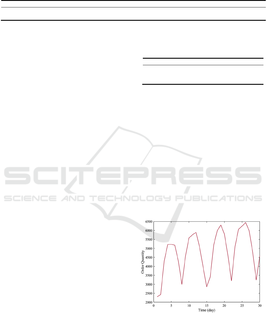
Table 1: Data records dictionary.

Field Name Description Example

tpep

pickup_datetime The time and date when the meter was turned on. 2023/3/1 0:06

PULocationID TLC Taxi Zone in which the taximeter was en

238

Search Algorithm (SSA), and Long Short-Term

Memory Networks (LSTM) to address the

shortcomings of traditional LSTM. The combination

of VMD and LSTM involves decomposing a time

series into multiple mode components, predicting

each mode's data separately using LSTM modeling,

and then combining the results to obtain the

prediction data. The coupling of SSA and LSTM

utilizes SSA to search for the optimal parameter

settings for the LSTM model. The VMD-SSA-LSTM

coupled model overcomes the limitations of a single

LSTM, significantly improving prediction accuracy.

This paper will use the publicly available dataset

of New York City's yellow taxi data, employing the

VMD-SSA-LSTM coupled model to predict the

demand for yellow taxis in February 2023. This will

enable us to obtain accurate future demand for yellow

taxis in various regions, facilitating proactive

scheduling and rational allocation of taxi resources in

different areas to achieve maximum efficiency.

2 METHODS

2.1 Data Sources

The dataset utilized in this article originates from the

open dataset on yellow taxi orders provided by the

Taxi and Limousine Commission (TLC) of New York

City. The dataset encompasses all yellow taxi order

data in New York City from January 1 to February

28, 2023. Fields including the vendor ID, the number

of passengers, the journey distance, the pickup and

drop-off locations, and the pickup and drop-off times

are all included in each order record. As this article

primarily focuses on predicting taxi demand, only the

pickup time and pickup location, are retained, as

illustrated in Table 1.

To ensure the accuracy and reliability of the

model, it is essential to perform data cleaning on the

raw dataset, removing inaccurate information and

fixing format errors. Inaccurate information can

introduce bias to the model, leading to a decrease in

precision and inaccurate predictions. For instance,

data points with timestamps outside of January 2023

or drop-off locations outside the designated areas may

compromise the model's performance. The data

sample after undergoing the cleaning process is

illustrated in Table 2.

Table 2: Example data.

p_p

icku

datetime PULocationID

2023/1/1 0:32 161

2023/1/1 0:55 43

2023/1/1 0:25 48

2.2 Preliminary Analysis of Data

After completing the data cleaning process to obtain

usable data, the initial step is to analyze the temporal

dimension to extract preliminary data features and

identify time-related patterns. In the temporal

analysis, this article focuses on the area with the

highest number of yellow taxi orders in New York

City, specifically the Upper East Side South (Zone

237). An analysis is performed on the yellow taxi

order volume in this area from January 1 to January

31, 2023.

The article begins by analyzing the daily yellow

taxi order data for January, as illustrated in Fig. 1. The

data exhibits a clear periodicity. With a weekly cycle,

the order volume reaches its lowest point on Sundays

and peaks from Wednesday to Friday.

Figure 1: The daily order quantity of yellow taxis for

January 2023 (Picture credit: Original).

Furthermore, the article conducts an hourly

analysis of the order quantity from January 9th to

January 11th, as depicted in Fig. 2. It is observed that

the order volume sharply increases around 7 AM each

Yellow Taxi Demand Prediction for New York City Based on VMD-SSA-LSTM

435

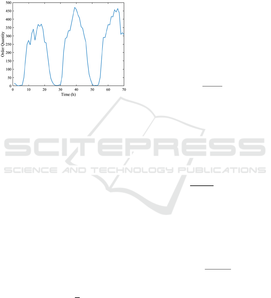
day, reaching its peak at approximately 2 PM. Taking

these two points into consideration, it is evident that

the distribution of taxi order data in this area, as a

commercially dense region, aligns with the observed

patterns.

Figure 2: The order quantity of yellow taxis from January

9th to 11th, 2023 (Picture credit: Original).

2.3 Variational Mode Decomposition

Variational Mode Decomposition (VMD) is an

adaptive, non-recursive technique for processing

signals and modal variation that may identify

pertinent frequency bands and estimate associated

modes on its own (Dragomiretskiy and Zosso 2013).

It demonstrates excellent performance in handling

stationary and nonlinear signals. One of its

advantages is the ability to determine the number of

decomposed modes, enabling the autonomous

separation of intrinsic modes. The objective is to

decompose the input signal f

into sub-signals μ

. It is

assumed that each mode μ

is predominantly compact

around its frequency center w

. The process can be

described in three steps.

Step one involves using the Hilbert transform to

get the analytic signal for every mode μ

In the second step, the center frequencies of each

mode are estimated, and the signals are demodulated

to the baseband.

In the third step, the Gaussian smoothness of the

signals is demodulated to estimate their bandwidth.

The following is the formulation:



min

















∑

𝜕



𝛿



𝑡









∗𝑢



𝑡







𝑠. 𝑡.

∑

𝑢





𝑡



𝑓



(1)

In this equation, µ

denotes the k modal

component, w

is the frequency center of the k mode,

and δ is the unit impulse function. Lagrange

multipliers λ and a quadratic penalty term are

included to prevent the issue from becoming

unconstrained. The alternate direction multiplier

approach is used to reach the final result.

2.4 Sparrow Search Algorithm

Sparrow Search Algorithm (SSA) is a revolutionary

intelligent optimization algorithm inspired by

sparrow populations' feeding and anti-predatory

activities (Xue and Shen 2020). It has the advantages

of quick convergence and high optimization

capabilities. The specific process is as follows.

Initialize the population and relevant parameters,

and calculate the initial fitness values of the

population.

Update the position of the discoverer:

𝑋

,



 

𝑋

,



exp













𝑅



𝑆



𝑋

,



𝑄𝑳 𝑅



𝑆



(2)

In this context, X

i,j

represents the position of the i-th

sparrow in the j-th dimension. α is a random number

with 𝛼∈0,1. iter

max

stands for the maximum

number of iterations, R

is a warning value within the

range 𝑅



∈



0,1



. S

represents the safety value and

lies within the range 𝑆



∈0.5,1. Q is a random

integer with a normal distribution, and L is a 1×D

matrix with all members set to 1.

The updated position of an entrant is given by the

following equation:

𝑋

,



 

𝑄∙exp 









,







 𝑖𝑛/2

𝑋





|𝑋

,



𝑋





| ∙𝑨



∙𝑳 𝑜𝑡ℎ𝑒𝑟𝑠

(3)

Here, 𝑋



represents the current discoverer's best

position, 𝑋

worst

is the current worst position, 𝑨 is a

matrix of size 1 𝐷 with randomly assigned values

of 1 or -1, and 𝑨







𝑨𝑨







The updated position of a sparrow that becomes

aware of the danger is given by the following

equation:

𝑋

,







𝑋





𝛽𝑋

,



𝑋





 𝑓



𝑓



𝑋

,



𝐾



,

























 𝑓



𝑓



(4)

Here, 𝑋



represents the globally best position,

𝛽 is a random number controlling the step size

following a normal distribution with mean 0 and

variance 1, 𝐾 is a random number with 𝐾∈1, 1,

𝑓



is the current individual fitness, 𝑓



is the current

global best fitness, 𝑓



is the current global worst

fitness, and 𝜀 is a constant.

ICDSE 2024 - International Conference on Data Science and Engineering

436

Calculate the fitness value, update the sparrow

positions, and assess whether the stopping criteria are

met. If the criteria are satisfied, output the results;

otherwise, return to step 2.

2.5 Long Short-Term Memory

A specific kind of Recurrent Neural Network (RNN)

called Long Short-Term Memory (LSTM) was

created to solve the problem of disappearing or

exploding gradients that occur when processing

lengthy sequential input. LSTM tackles this problem

by introducing gate structures and a cell state. An

input gate, an output gate, and a forget gate make up

the gate structures. The cell state permits the long-

term storage of information, and these gates

efficiently regulate the flow of information in and out.

The forget gate determines how much of the cell

state information to discard and is formulated as

follows:

𝑓



𝜎𝑤



∙



ℎ



, 𝑥





𝑏



 (5)

where 𝑤



is the weight matrix, 𝑏



is the bias

term, ℎ



is the hidden state from the previous time

step, 𝑥



is the current input, and 𝜎 is the sigmoid

function.

The input gate decides which new information to

store in the cell state and consists of two components:

𝐶



𝑡tanh 𝑊



∙



ℎ𝑡1, 𝑥





𝑏



 (6)

𝑖



𝜎𝑊



∙



ℎ



, 𝑥





𝑏



 (7)

where 𝑊



and 𝑊



are weight matrices, 𝑏



and 𝑏



are biased terms, ℎ



is the hidden state from the

previous time step, 𝑥



is the current input, 𝜎 is the

sigmoid function, and tanh is the hyperbolic tangent

function.

Based on the forget gate and input gate, the

memory cell is updated using the formula:

𝐶



𝑓



∗𝐶



𝑖



∗𝐶



𝑡 (8)

where 𝑓



is the forget gate output, 𝐶



is the

previous time step cell state, 𝑖



is the input gate value,

and 𝐶





is the candidate's value.

The output gate determines the information to

output based on the cell state, and its formula is:

𝑜



𝜎𝑊



∙ℎ



, 𝑥



𝑏



 (9)

ℎ



𝑜



∗tanh 𝐶



 (10)

Where 𝑊



is the weight matrix, 𝑏



is the bias

term, ℎ



is the hidden state from the previous time

step, 𝑥



is the current input, 𝜎 is the sigmoid function,

𝐶



is the current cell state, and tanh is the hyperbolic

tangent function.

LSTM performs forward propagation through

these processes and then utilizes the computed results'

errors for backward calculation, updating the weights

until the maximum iteration is reached.

2.6 VMD-SSA-LSTM

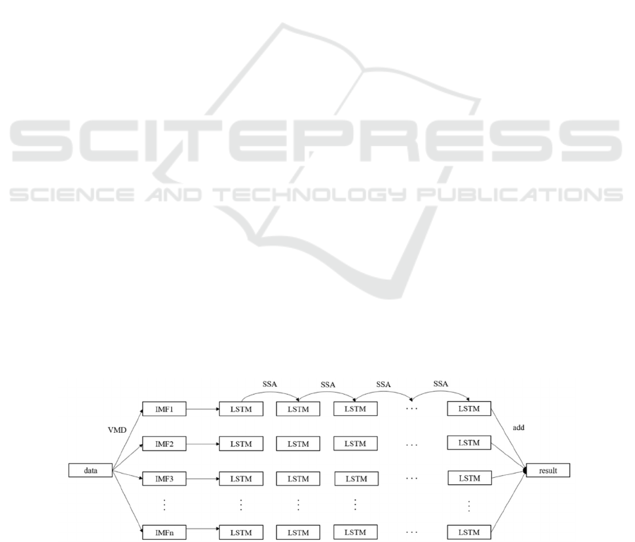
To integrate the three aforementioned methods into

the VMD-SSA-LSTM network for taxi demand

prediction, the model schematic is depicted in Fig. 3.

The specific process involves the following steps.

1) Selecting a suitable time duration for the data

and determining the time granularity. After adding up

all of the orders for each time period, divide the

dataset into training and testing sets.

2) Decomposing the dataset into k components

using the VMD method. To prevent data leakage,

isolate the testing set, and decompose the training set

separately.

3) Determining the learning rate, the number of

training iterations, and the number of hidden layer

neurons for the SSA optimization. Select the

maximum number of iterations and the population

size for the SSA. A linked model of the SSA and

LSTM is established by using the mean squared error

as the optimization objective function.

4) Applying the SSA-LSTM model to forecast

every mode separately. To estimate taxi demand, get

projections for k components and add them together.

Figure 3: VMD-SSA-LSTM coupled model schematic chart (Picture credit: Original).

Yellow Taxi Demand Prediction for New York City Based on VMD-SSA-LSTM

437

3 RESULTS AND DISCUSSION

3.1 VMD and SSA Results

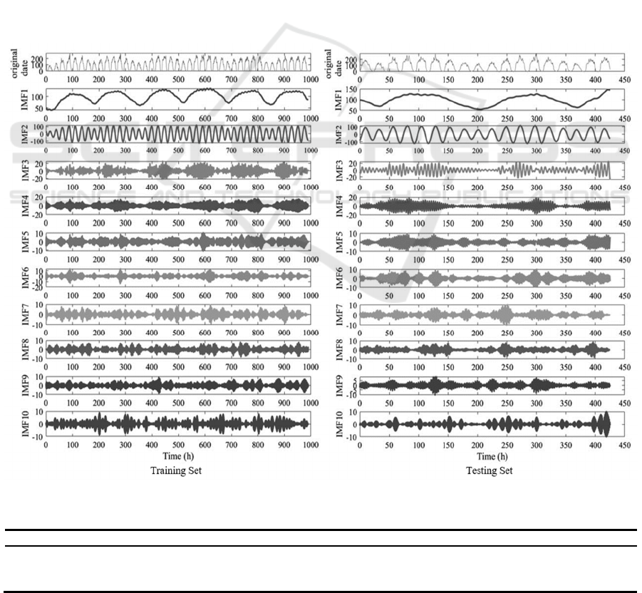
Firstly, the dataset undergoes VMD to determine the

appropriate number of decomposition components,

denoted as k. A stepwise selection is used to test

values, incrementally increasing until the central

frequencies of the final decomposed variables

stabilize. The value of k corresponding to the stable

point is selected, with a choice of k = 10 in this case.

To prevent data leakage, start by extracting data

corresponding to the training set from the dataset.

Break down this subset to create decomposed training

set data. Subsequently, decompose the entire global

dataset. Then, extract data corresponding to the test

set time points to generate decomposed test set data.

The decomposed data is shown in Fig. 4. VMD

has separated the training and test sets into ten

different frequency modes, extracting various

periodic components and uncovering implicit

patterns and noise within the time series.

The SSA is configured with a sparrow quantity of

10, a maximum iteration count of 10, 3 optimized

parameters, an alert value of 0.6, an inclusion ratio of

0.3 for newcomers, and a count of sparrows that

become aware of danger set at 0.2. Optimization

process is initiated to search for the optimal LSTM

model parameters, resulting in the following

outcomes: the optimal number of hidden units is 185,

the optimal maximum training epochs is 199, and the

optimal initial learning rate is 4.713×10

(-3)

3.2 Prediction Results and Comparison

In this study, VMD-SSA-LSTM is employed for taxi

demand forecasting, and it is compared with LSTM

and VMD-LSTM. The evaluation metrics for

assessing model performance include Root Mean

Square Error (RMSE), Mean Absolute Error (MAE),

and Mean Absolute Percentage Error (MAPE).

Figure 4: The VMD results for the training set and testing set (Picture credit: Original).

Table 3: Testing set errors for the three methods.

Model RMSE MAE MAPE

LSTM 23.157 18.103 13.213%

VMD-LSTM 12.517 9.612 7.658%

VMD-SSA-LSTM 5.075 4.274 3.074%

ICDSE 2024 - International Conference on Data Science and Engineering

438

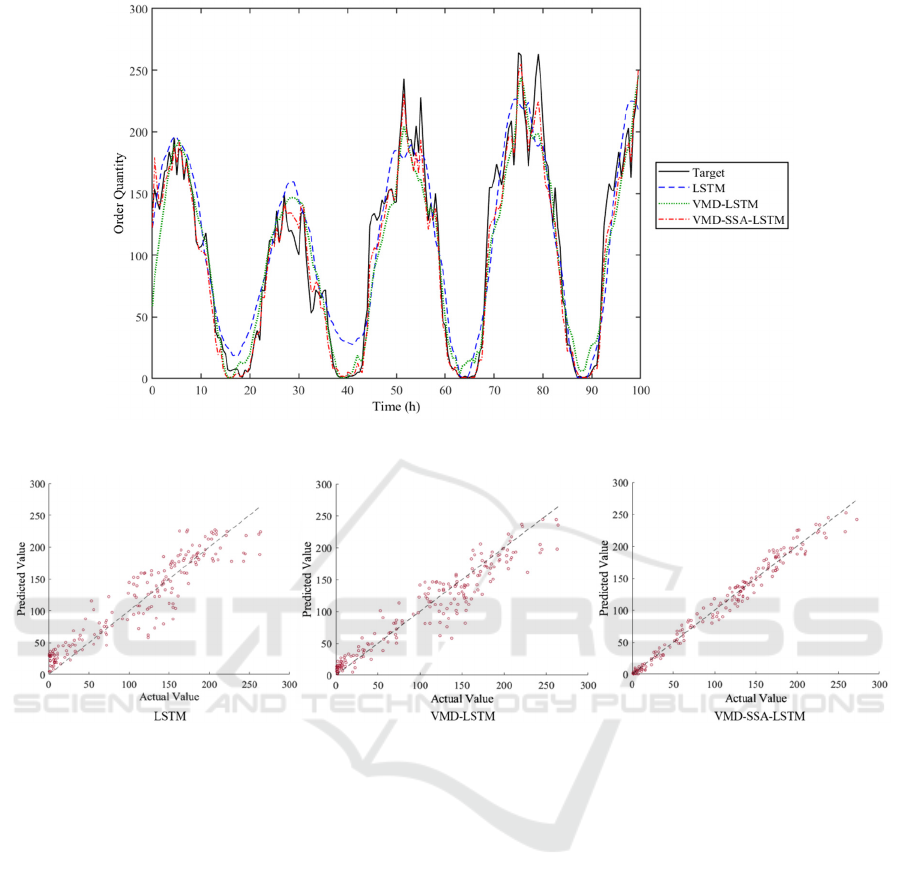
Figure 5: Testing set predictions for the three methods (Picture credit: Original).

Figure 6: Scatter plot of testing set predictions and original data for the three methods (Picture credit: Original).

The errors on the test set for the three methods are

summarized in Table 3. It is apparent from the table

that VMD-SSA-LSTM demonstrates superior

performance compared to both LSTM and VMD-

LSTM, achieving a remarkable reduction of 78.1%

and 59.5% in RMSE, respectively. In addition, there

is a noticeable decrease in both MAE and MAPE.

The predicted results for the three methods on the

test set have been graphically represented over time

in Fig. 5. As depicted in the figure, the predictive

performance of VMD-SSA-LSTM stands out as

superior, followed by VMD-LSTM. In contrast, the

standalone LSTM model exhibits comparatively

lower predictive capabilities. This disparity is

attributed to the LSTM model's lower complexity

compared to the other two coupled models, leading to

less refined data processing.

A scatter plot, illustrating the comparison between

test set predictions and the original data for the three

methods, is presented in Fig. 6. The figure clearly

indicates that, when contrasted with VMD-LSTM,

VMD-SSA-LSTM exhibits superior overall

performance, particularly showcasing accurate

predictions when dealing with larger numerical

values.

In summary, there are two notable issues with

LSTM in the context of taxi demand forecasting.

Firstly, it exhibits poor performance when predicting

long sequence data, possibly due to overfitting or a

failure to capture implicit relationships within the

time series data. Secondly, determining model

parameters for effective prediction proves

challenging, leading to suboptimal results. By

employing VMD for denoising data and extracting

latent information from time series data, and

subsequently using SSA to search for optimal LSTM

model parameters, these issues are addressed.

Ultimately, the coupled VMD-SSA-LSTM network

proves to be highly accurate in forecasting taxi

demand.

Yellow Taxi Demand Prediction for New York City Based on VMD-SSA-LSTM

439

4 CONCLUSION

This paper explores the taxi order data of yellow cabs

in New York City from January to February 2023.

Firstly, the data is processed and subjected to simple

analysis to derive statistical information and identify

patterns. Subsequently, a coupled VMD-SSA-LSTM

network is employed for taxi demand forecasting, and

the outcomes are contrasted with those obtained using

LSTM and VMD-LSTM.

The results display that the coupled model

demonstrates a more accurate predictive

performance. The final RMSE for the coupled

model's predictions is 5.075, which represents a

reduction of approximately 80% compared to the

single LSTM's 23.157. The coupled models exhibit a

higher level of refinement in data processing,

enabling more accurate predictions of the trend in

order data. VMD and SSA effectively address the

shortcomings of LSTM in handling time series data

with insufficient precision and challenging parameter

determination.

This coupled model exhibits excellent

performance in predicting the demand for yellow

taxis in New York City, and its application could be

extended to short-term passenger flow predictions in

other areas. Additionally, exploring more

sophisticated optimization algorithms may yield even

more precise results in the future.

REFERENCES

D. Cao, K. Zeng, J. Wang, IEEE Transactions on Intelligent

Transportation Systems, 23(7): 9442-9454 (2021).

K. Zhao, D. Khryashchev, H. Vo, IEEE Transactions on

Knowledge and Data Engineering, 33(6): 2723-2736

(2019).

X. L. Zhang, G. He, H. Lu, Journal of Systems Engineering,

24(2): 178-183 (2009).

Z. S. Yao, C. F. Shao, Y. L. Gao, Journal of Beijing

Jiaotong University, 30(3): 19-22(2006).

S. Sun, C. Zhang, G. Yu, IEEE Transactions on Intelligent

Transportation Systems, 7(1): 124-132 (2006).

J. Xu, R. Rahmatizadeh, L. Bölöni, et al., IEEE

Transactions on Intelligent Transportation Systems,

19(8): 2572-2581 (2017).

Y. Lai, K. Zhang, J. Lin, Taxi demand prediction with

LSTM-based combination model, in Proceedings of

2019 IEEE Intl Conf on Parallel & Distributed

Processing with Applications, Big Data & Cloud

Computing, Sustainable Computing &

Communications, Social Computing & Networking

(ISPA/BDCloud/SocialCom/SustainCom), 944-950.

K. Zhao, D. Guo, M. Sun, IEEE Access, 97072-97088

(2023).

H. Li, Y. Zhao, C. Ma, Journal of Advanced Transportation,

2022 (2022).

K. Dragomiretskiy, D. Zosso, IEEE transactions on signal

processing, 62(3): 531-544 (2013).

J. Xue, B. Shen, Systems Science & Control Engineering,

8(1): 22-34 (2020).

ICDSE 2024 - International Conference on Data Science and Engineering

440