Reliability Analysis of Francis Turbine Cracking Using Gamma Frailty

Model and Censored Historical Maintenance Data

eophile Mbuyi Tshibangu

, Guyh Dituba Ngoma

, Martin Gagnon

and S

ebastien Carle

School of Engineering, University of Quebec in Abitibi-T

emiscamingue, 445 Boulevard de l’Universit

e, Rouyn-Noranda,

J9X 5E4, Canada

Hydro-Qu

ebec’s Research Institute, 1800, boulevard Lionel-Boulet, Varennes, Quebec, J3X 1S1, Canada

Hydro-Qu

ebec, 1095 Rue Saguenay, Rouyn-Noranda, Quebec, J9X 5B5, Canada

Keywords:

Gamma Frailty Model, Reliability, Cracks, Hydraulic Turbine, Censored Historical Data.

Abstract:

All over the world, the need for electrical energy has increased dramatically, forcing hydroelectric power plants

to operate under non-standard conditions. This leads to premature fatigue cracking and consequently to multi-

ples crack inspections. In this research, a probabilistic model is developed based on frailty and censoring. The

model takes advantage of the use of a Non-Homogeneous Poisson Process (NHPP) because turbine runners

are considered as repairable parts. We develop the marginal likelihood expression incorporating frailty effect

using gamma frailty distribution and we use the stochastic gradient descent (SGD) algorithm to obtain the

optimal parameters. Furthermore, instead of considering the frailty effect z as a random variable, we decide

to derive its expression from the individual unconditional likelihood function that has been also optimized.

Finally, we compare reliability and cumulative hazard functions between family members. We then conﬁrm

the results obtained by comparing reliability between two families that behaved differently. Results shows

that frailty effect, that is fonction of failure statuses and individual ﬁnal time of observation for a speciﬁc

component has played an impor tant role in differentiating heterogeneity among groups of the same family.

Reliability curves clearly demonstrate heterogeneity within and between families.

1 INTRODUCTION

Industrial development throughout the world and even

daily life of human beings have become largely de-

pendent on electrical energy. Among electricity pro-

duction methods, hydropower represents less than

20% of global production (Liu et al., 2016a; Trivedi

and Cervantes, 2017). However, it far exceeds other

forms of green energy production combined. The

availability of turbine runner and alternator units is

therefore essential, especially in region such as Que-

bec with limited potentials in other forms of renew-

able energy. Hydro-Qu

ebec, the electricity produc-

tion compagny in Canada, with a ﬂeet of 60 hydro-

electric power plants, saw a drop in electricity sales

from 216.2 TWh in 2022 to 200.3 TWh in 2023

(Hydro-Qu

ebec, 2023). Cavitation and cracks that ap-

pear on some turbine runners families, limit the avail-

ability of the units and consequently increase main-

tenance costs, as well as the number of shutdowns

and start-ups due to systematic inspections and re-

pairs. However, these transient zones of start-ups and

shutdowns are generally responsible of turbine crack-

ing because of high stress ﬂuctuations (Morin et al.,

2021). On the other hands, some families are run in

off-design conditions to maintain the demand in elec-

trical energy (Morin et al., 2021).

Basically, a turbine runner is designed to with-

stand fatigue damage. Unfortunately, fatigue cracks

appear as a random effects (Georgievskaia, 2020) in

some turbine runners families. Researchers have been

scrambling to identify the principal causes of these

cracks (Liu et al., 2016b) as indicated in Figure 1. An-

alytical, physical, numerical and data based models

were developped. For example, (Morin et al., 2021)

analysed the transients effects on the lifespan of tur-

bine runner. They concluded that the startup, shut

down and time of speed no load create ﬂuctuations

that lead probably to cracks. (Gagnon et al., 2010)

evaluated the ﬂuctuations of the stresses at the start-

up in order to optimize the life expetancy of a turbine

runner. (Thibault et al., 2015) examined the material

properties especially 13% Cr-4%Ni stainless.

Furthermore, site expreriments and campaign mea-

128

Tshibangu, T., Ngoma, G., Gagnon, M. and Carle, S.

Reliability Analysis of Francis Turbine Cracking Using Gamma Frailty Model and Censored Historical Maintenance Data.

DOI: 10.5220/0012813000003758

Paper published under CC license (CC BY-NC-ND 4.0)

In Proceedings of the 14th International Conference on Simulation and Modeling Methodologies, Technologies and Applications (SIMULTECH 2024), pages 128-137

ISBN: 978-989-758-708-5; ISSN: 2184-2841

surements have been used to evaluate reliability

(Trivedi et al., 2013). For instance, (Gagnon et al.,

2014) made strain measurement and used operation

history to capture reliability of turbine runners. (Ba-

jgholi et al., 2021) evaluated the use of advanced ul-

trasonic inspection to learn about the manufaccturing

ﬂaws and cracks. (Bajgholi et al., 2023) evaluated

reliability by using a non destructive testing to cap-

ture manufacturing ﬂaws. In addition, (Wang et al.,

2012), (Zhang et al., 2019) discovered that the man-

ufacturing ﬂaws in runner blades such as heterogene-

ity, anisotropic character and thinning of blade thick-

nesses could be the cause of cracking when runner is

working under critical conditions.

These studies have been done based on simpliﬁed

physical models simulations or standard measure-

ments. However, ﬁnding a model that incorporates the

complexity of all the predominant causes would be a

major challenge, as the various causes cannot be com-

bined in a physical model (residual stresses, transient

conditions, manufacturing ﬂaws, etc.) (Xiao et al.,

2010, Xiao et al., 2008) . In addition, experimental

measurements have given results quite different with

what were really observed in hydroelectric plant.

Figure 1: Cracks on Francis runner blades.

Another approach is the use of probabilistic model

based on operational hydroelectic site data to appre-

hend crack initiation (Gagnon et al., 2014). For in-

stance, (Georgievskaia, 2021) run an algorithm using

operational data to predict the remaining lifetime for

turbine runners that were above 30 years old. These

measurement processes are essentially costly when it

comes to monitoring each individual turbine runner.

The third approach is based on experience. This

approach makes use of historical maintenance data

to evaluate reliability of components. For example,

(Ivanchenko and Prokopenko, 2020) analyzed cracks

on turbine blades based on failure history. They found

that residual stresses and internal defects in the mate-

rial promote cracking. They predict the possible loca-

tion of the crack according to maintenance data and

show that reliability is decreasing with the age.

This study is also based on the processing of real

historical maintenance data for two turbine families.

The main objective is to develop a probabilistic model

that can reﬂect what is actually observed in hydroelec-

tric power plants. To do this, we build a model that

incorporates the individuality of each turbine in terms

of its frailty effect, and use censored maintenance data

to capture the reliability information stored in preven-

tive inspections and crack observations. By classify-

ing individuals with similar reliability trends, we can

decide whether to reduce unnecessary systematic in-

spections or monitor just one of the individuals of the

same type with similar reliability trends. The choice

of two different families will enable us to validate the

robust family and the most vulnerable one observed.

2 FRAILTY MODEL

Simulations done by (Gagnon and Nicolle, 2019)

demonstrate that non-uniformities and excentricities

of a turbine runner assembly could affect the dynamic

behaviour among the same family. This combined

with manufacturing varaibilities make each turbine

unique and explain the fact that cracks do not appear

in the same way among the family members. Hence,

turbine runners could not be considered as homoge-

nous in the same family. Futhermore, turbine runners

that were repaired and welded will show different be-

haviour. All these factors demonstrate that each tur-

bine runner is unique and has its own frailty. Frailty

is an unobserved covariate or a random effect that can

not be measured but affects the reliability in the model

(Therneau et al., 2003).

Indeed, the behaviour of a repairable component

can be captured in historical maintenance data, and

can lead to a frailty parameter that distinguishes com-

ponents from each other, even if they belong to the

same family. One of the best methods is to optimize

censored maintenance data using a survival analysis

model.

2.1 Censoring

Censoring generally communicates partial informa-

tion on the observation of the event. When a visual in-

spection is carried out and no crack (fatigue damage)

is detected, this information is censored (Wienke,

2010).

Let us consider a repairable entity with observation

times t

, . . . ,t

which could be inspection or repair

times, let t

∗

, ..., t

∗

be the survival times when fail-

ure occurs (crack detected) and c

, c

, ..., c

be the

censored times (no crack detected). At each obser-

Reliability Analysis of Francis Turbine Cracking Using Gamma Frailty Model and Censored Historical Maintenance Data

129

vation, we will have the couple (t

, δ

) (Munda et al.,

2012) such that:



1 when t

∗

≤ c

, t

is not censored

0 when t

∗

> c

, t

is censored

(1)

Each δ represents a failure status, indicating

whether or not the crack was observed at the time of

the event (crack inspections during cavitation repair,

systematic inspections or crack detection).

2.2 Stochastic Process

There are mathematical probabilistic models that can

be used to process time-dependant data to obtain

a distribution. These models differ depending on

whether the observation data are for a repairable en-

tity or not (Ascher, 2008).

A non-repairable entity has a unique lifetime. It is

replaced once the failure has occurred. The reliability

of this type of entity can be modeled by probabilistic

mathematical distributions such as Kaplan Meier, ex-

ponential distribution, Weibull’s distribution (Asfaw

and Lindqvist, 2015). Some repairable components

can be replaced when the cost of maintenance be-

comes too excessive. In this case, they are considered

and modeled as non-repairable components. Mainte-

nance activities on a repairable entity can either bring

it back to the state where it looks new (as good as

new) by improving the reliability, or back to the state

it was before the failure was observed (as bad as old)

(Love and Guo, 1991),(Ascher, 1968) .

Several stochastic processes exist for repairable

entities (Slimacek and Lindqvist, 2016):

- Renewal Process (RP)

- Homogeneous Poisson Process (HPP)

- Nonhomogeneous Poisson Process (NHPP)

- Branching Poisson Process (BPP)

In literature, NHPP is most suitable for repairable

entities in which failures occur randomly (Slimacek

and Lindqvist, 2016). Therefore, the minimal repair

assumption is used which means that after repair, the

reliability still decreasing as if failure were not ap-

peared. Several mathematical laws exist to model

a NHPP. However, the power law remains the most

practical (Oliveira et al., 2013),(Brown et al., 2023).

The baseline hazard function of the power law is

given in Equation 1.

(t) = ωρt

ρ−1

(2)

with ω the scale parameter and ρ the shape parameter

of the curve.

If ρ > 1, the system is deteriorating (sad system),

If 0 < ρ < 1, the system is improving (happy sys-

tem)

If ρ = 1, the failure intensity function is a constant

and the model can be used in a HPP process with the

exponential distribution.

2.3 Frailty Distribution

In survival analysis, several models are not giving ex-

pected results for the fact that heterogeneity effect

was not taken into account. Incoporating frailty in

the model allows to consider both random effects and

unobservable heterogeneity in the survival analysis.

Let z be a positive time-independent random fac-

tor that acts multiplicatively on the intensity function.

We assume that the z is time-independent and is re-

lated to each entity. However, this factor, in general,

can also vary over time depending on certain criteria

or the data of the problem. The intensity function with

frailty effect is:

h(t) = zωρt

ρ−1

(3)

z > 1 means that failure will often occur and z < 1

leads to less failure occurence (Vaupel et al., 2023).

In case we will ﬁnd z = 1,this means that the compo-

nents have no heterogeneity and can only be modelled

by a power law without frailty effect. In addition,

components with z = 0 fragility refer to those with

higher reliability, especially when nothing is recorded

to classify them.

The random variable z is expected to follow a spe-

ciﬁc probability distribution. Let f (z) be the frailty

probability density function of z. For time-event

data, several univariate frailty models exist. The most

widely used are the Gamma frailty and inverse Gaus-

sian frailty models. However, the Gamma frailty dis-

tribution is the most popular because of the gamma

function’s mathematical properties and computational

aspects (Asfaw and Lindqvist, 2015).

2.3.1 Gamma Frailty Distribution

(Duchateau and Janssen, 2008), (Brown et al., 2023),

(Asfaw and Lindqvist, 2015) used gamma distribution

to model heterogeneity. (Abbring and Berg, 2007)

has revealed that in most cases, for a large class, the

frailty distribution converges to a gamma distribution

as time approaches inﬁnity. As we are using data

for turbine runner that approach to end of lifetime,

we have considered gamma frailty distribution in the

model. In the literature, the likelihood comparison

of the data obtained with frailty gamma distribution

gave better results compared to traditional parametric

models (Brown et al., 2023). The probability density

function of the gamma distribution is :

f (z) =

Γ(k)

k−1

−λz

(4)

SIMULTECH 2024 - 14th International Conference on Simulation and Modeling Methodologies, Technologies and Applications

130

with λ the inverse scale parameter and k the shape

parameter. Using the Lapace transform and mathe-

matical properties of gamma function, we can show

that the mean and variance of the gamma distribution

respectively are

var(z) =

(5)

and

E(z) =

. (6)

With z being a positive number. Let assume that

the mean of the gamma distribution is unit and let call

the variance by θ. Therefore k =

= λ. The probal-

ity density function for gamma frailty distribution be-

comes:

f (z) =

Γ(

)

(

)

−1

−

(7)

2.3.2 Likelihood Function

One of the best way for determinimg different param-

eters of the frailty model that could highly ﬁt with

data is to optimize the likelihood function. Let j be

a repairable entity with a ﬁnite number of failures n

with j = 1, 2, . . . , m components in the system. The

conditional likelihood function for this entity is given

by:

i j

)|z

) =

∏

i=1

i j

))

i j

. . .

×exp[−z

(τ

) − H

))]

(8)

with H

(t) the cumulative hazard function given in

Equation (9).

(t) = ωt

(9)

and S

represent respectively the ﬁnal and the start-

ing times of the observation period for the component

j. Let assume that S

= 0 day as an initial time for the

model.

The conditional likelihood function for this com-

ponent with respect to z

is given in the equation (10).

(θ|h

i j

)) =

∞

∏

i=1

i j

))

i j

. . .

×exp(−z

(τ

)) f (θ|z

)dz

(10)

By replacing gamma distribution and using

gamma function properties, the marginal or uncondi-

tional likelihood function for component j is

(ω, ρ, θ) =

∏

i=1

i j

))

i j

Γ(d

)θ

Γ(

)[θH

(τ

) + 1]

)

(11)

with d

∑

i=0

i j

Equation (11) was developed in this study and is

of great importance as it takes into account the frailty

effect, censored data and the stochastic process of re-

pairable components, the NHPP. This increases the

probability of having a model that matches the histor-

ical maintenance data and will enable vital informa-

tion to be extracted. Moreover, instead of simplifying

the model by considering the ﬁnal time τ

as a con-

stant for all components as seen in the literature, we

manage to keep it individual in order to model the ex-

act effect of the heterogeneity that differentiates the

components.

For m components in the system, the total likeli-

hood function is the sum of likehood function for each

component. Therefore, the marginal likelihood func-

tion for the system is:

L =

∑

j=0

(ω, ρ, θ) (12)

The simplest way to handle this complex expres-

sion is to use the logarithmic function. Therefore, the

logarithm of the marginal likelihood function for m

components is

marg

∑

j=1

∑

i=1

i j

(logω + logρ + (ρ − 1)log(t

i j

))

. . .

∑

j=1



logΓ(d

) + d

log(θ) − log(Γ(

))



. . .

−

∑

j=1



)log(θωτ

+ 1)



(13)

The maximum of the marginal likelihood function

is the value at which parameters (ω, ρ, θ) are opti-

mums. Let ﬁnd the partial derivative of marginal like-

lihood with respect to each parameter of the model.

Equations (14,15,17) give these partial derivatives.

∂l

marg

∂ω

∑

j=1

∑

i=1

i j

. . .

−

∑

j=1

(1 + θd

)

1 + θωτ

(14)

∂l

marg

∂ρ

∑

j=1

∑

i=1

i j

(

+ log(t

i j

))

. . .

−

∑

j=1

(1 + θd

)

ωτ

logτ

1 + θωτ

(15)

Reliability Analysis of Francis Turbine Cracking Using Gamma Frailty Model and Censored Historical Maintenance Data

131

Deﬁne number of iteration N

Deﬁne number of components m

Deﬁne the learning rate α

Deﬁne initial values of parameters ω

, ρ

, θ

Data: Input t

i j

, τ

, δ

i j

, n

while k < N do

while j < m do

while i < n

compute expressions in marginal

likelihood and partial derivatives

function starting from i=1 to n

;

end

compute expressions in marginal

likelihood and partial derivatives

function starting from j=1 to m ;

end

marg

(ω

, ρ

, θ

);

grad

∂l

marg

∂ω

(ω

, ρ

, θ

);

grad

∂l

marg

∂ρ

(ω

, ρ

, θ

);

grad

∂l

marg

∂θ

(ω

, ρ

, θ

);

k+1

= ω

+ α × grad

;

k+1

= ρ

+ α × grad

;

k+1

= θ

+ α × grad

end

Result: Plot l

marg

Result: Print (ω

, ρ

, θ

), with l the index of

maximal value of l

marg

Algorithm 1: Stochastic Gradient Descent Algorithm.

The partial derivative with respect to θ is done us-

ing the property of derivative of log Γ(u) which in-

volves the use of digamma function 𭟋(u) such as

logΓ(u) =

′

(u)

Γ(u)

= u

′

𭟋(u)

(16)

Using Equations (13) and (16), the partial deriva-

tive of the logarithm of the marginal likelihood func-

tion with respect to θ is

∂l

marg

∂θ

∑

j=1



−

𭟋(d

) +

𭟋(

)



. . .

∑

j=1



log(1 + θωτ

)



. . .

−

∑

j=1

)

ωτ

1 + θωτ

(17)

In this study, we use the stochastic gradient decent

(SGD) algorithm for optimizing the likelihood func-

tion, as it is a Newton-Raphson method that has given

better results in the literature (Haji and Abdulazeez,

2021, Mercier et al., 2018).

Algorithm 1 gives details on the stochastic gradi-

ent descent method used for this study. We ﬁrst deﬁne

all functions and compute them at each step of itera-

tion and get optimum parameters at maximum likeli-

hood value for a speciﬁc family.

Finally, we calculate the frailty parameter z, the

cumulative hazard function and the reliability func-

tion. These functions enable us to classify the risk

of cracking within a family. A comparison between

two turbine families is adopted to validate what has

been observed: turbine runners (groups) from family

B crack more than those from family A. We therefore

used the same length of observations for both fami-

lies.

2.3.3 Frailty Parameter

Previous research has treated z as a random variable.

In this study, as we are motivated to compare the

risk of cracking between individuals, we adopt an-

other approach to derive the value of z immediately

from censored data. From equation (8), we can obtain

the frailty parameter that maximizes the conditional

likelihood function L

. The logarithm of the condi-

tional likelihood function L

for a speciﬁc component

is given by equation (18).

log(L

(ω, ρ, θ)) =

∑

i=1

i j

(log(z

) + log ω + log ρ

. . .

∑

i=1

i j

+ (ρ − 1) log(t

i j

))

− z

ωτ

(18)

Consequently, the optimal frailty parameter that

expresses the data for the j component is obtained by

calculating the partial derivative of Equation (18) with

respect to z

and equalizing it to zero. This yields

∑

i=1

i j

ωτ

(19)

Equation (19) reveals that z

is highly dependent

on the failure status data δ

i j

and the ﬁnal event time

for component j. If no failure is recorded during the

observation period, the value of z

equals zero and

frailty distribution can no longer be used for that spe-

ciﬁc component. However, the contribution of that

component with zero frailty have been included in the

overall system model in the marginal likelihood ex-

pression.

2.3.4 Reliability

With the parameters of the model and frailty effect, it

is easier to compute the unconditionnal reliability of

SIMULTECH 2024 - 14th International Conference on Simulation and Modeling Methodologies, Technologies and Applications

132

the component j as given in Equation (20).

(t|z

) = exp(−z

ωt

) (20)

In addition, the marginal reliability function for

the same component is given by

(t) =

∞

f (z

;θ)exp(−z

ωt

)dz

(21)

3 SIMULATIONS

3.1 Events Data

To validate the model, we choose two different fami-

lies of turbine runners. Family A has reliable groups

than family B. We also choose the same observa-

tion period to compare the curves of the two fami-

lies. Within the same family, the frailty effect will

play a role in differentiating turbine runners. This

will enable comparisons to be made within and be-

tween families. The data used for simulations are the

real observation times (inspections and crack repairs)

and failure statuses for ten Francis turbine runners be-

longing to families A and B. The failure statuses pro-

vide information on censoring. The observation pe-

riod runs from January 2001 to January 2022. Data

are collected from the maintenance history database.

Tables 1 and 2 show the age in years of the ten groups

at the start of the observation period.

Table 1: Age for groups in family A (years).

GR 01 GR03 GR05 GR07 GR10

19 19.5 19.7 20 21.2

Table 2: Age for groups in family B (years).

GR 01 GR03 GR05 GR07 GR10

19.4 19.5 20 20.1 21.4

Table 3 gives the observed event times for family

A, and the corresponding failure statuses are in Table

In the same way, table 5 contains recorded event

times data for family B and the corresponding failure

statuses are in Table 6.

3.2 Results and Discussion

We use the SGD algorithm described in section 2.3.2

and the data in section 3.1. The learning rate is 0.0071

for both families. The initial parameters used for fam-

ilies A and B are given in Table 7.

Table 3: Event times for groups in family A (days).

GR 01 GR03 GR05 GR07 GR10

1304 1739 674 737 369

1403 3057 1373 2199 1102

1892 3427 1495 2483 2602

3427 3708 1556 3427 3393

3680 6701 2314 3708 3617

4009 2347 5036

5593 3057

6236 3176

3427

3708

4394

5575

Table 4: Failure Statuses for groups in family A.

GR 01 GR03 GR05 GR07 GR10

0 0 0 0 0

1 0 0 0 1

0 0 1 0 1

0 0 0 0 0

1 0 0 0 0

0 1 0

0 0 0

0 0

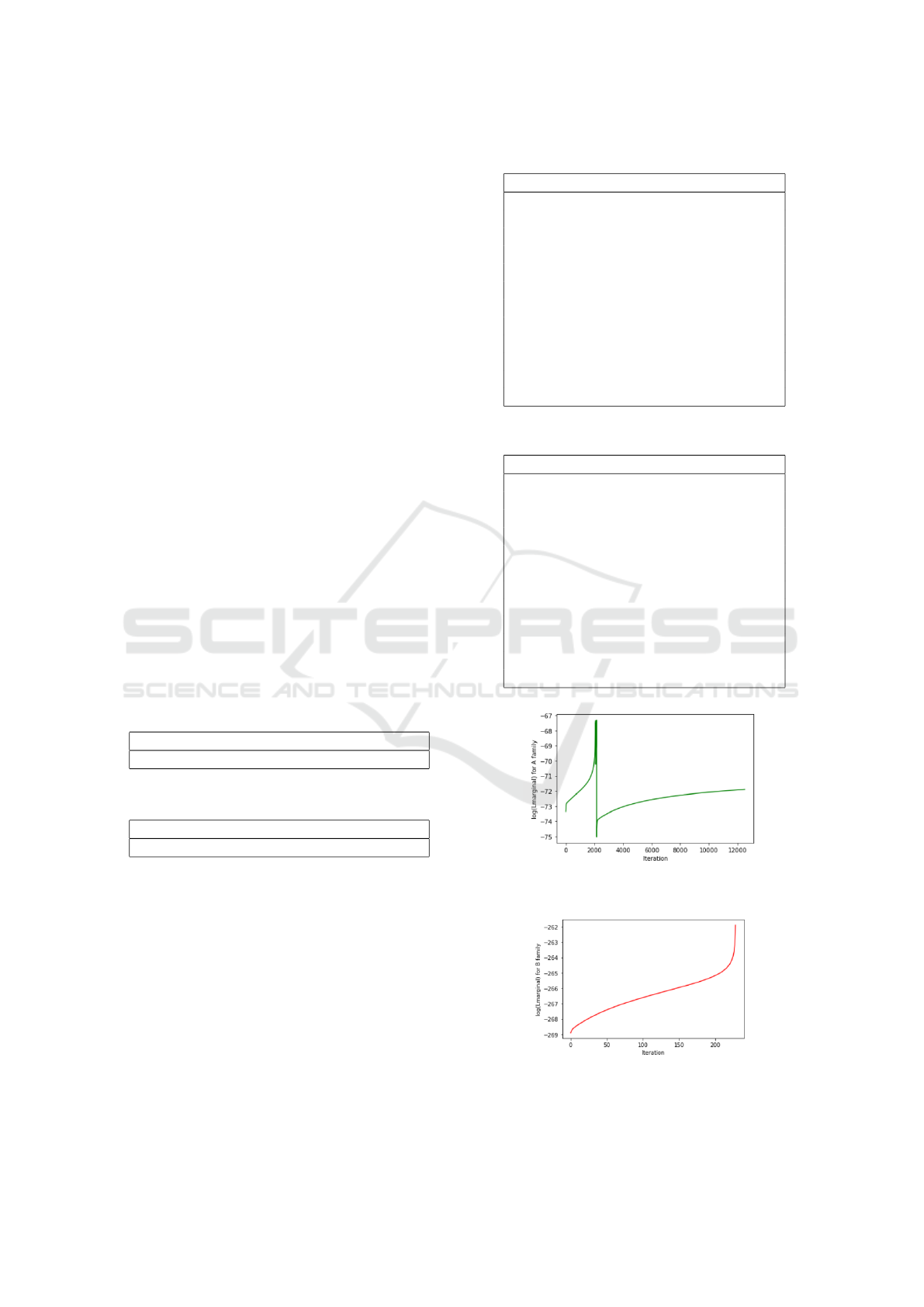
Figure 2: Evolution of the logarithm of the marginal likeli-

hood function for family A.

Figure 3: Evolution of the logarithm of the marginal likeli-

hood function for family B.

Reliability Analysis of Francis Turbine Cracking Using Gamma Frailty Model and Censored Historical Maintenance Data

133

Table 5: Event times for groups in family B (days).

GR 02 GR04 GR06 GR08 GR09

292 794 947 347 823

613 1283 1102 766 977

895 1495 1523 947 1495

1403 1768 2255 1130 2227

1892 2089 2497 1201 2868

2347 2588 2679 1710 3232

2658 2889 2854 2227 3624

2777 3202 3099 2595 4062

3260 3379 3253 2847 4412

3687 3533 3638 3134 4636

3722 4002 4051 3561 4715

3911 4379 4410 3981 5085

4445 4711 4051 4392 5441

4716 4755 4442 5469

5184 5195 4606 5777

5423 5406 5040 6081

5709 5816 5830 6238

6311 6311

6660 6531

6733 6965

7091 7336

Table 6: Failure statuses for groups in family B.

GR 02 GR04 GR06 GR08 GR09

1 0 0 1 0

0 0 1 1 0

0 0 0 0 0

1 0 0 1 0

0 1 0 0 0

0 0 0 1 0

0 0 0 0 1

1 0 0 0 0

0 0 0 0 0

1 0 0 0 1

0 1 0 0 0

1 0 1 1 0

1 1 0 1

1 0 0 0

1 1 1 1

1 1 1

1 1

1 0

0 0

After running the algorithm, Figure 2 illustrates

the evolution of the logarithm of the marginal like-

lihood function for family A , and the correspond-

ing optimal parameters obtained are shown in Table

8. Similarly, the algorithm run for family B groups

Table 7: Initial parameters of the model.

ω ρ θ

Family A 2 0.5 3

Family B 2 1.0 3

gives the evolution of the logarithm of the likelihood

function in Figure 4, and the corresponding optimal

parameters are in table 9. In Figure 3, we have a sin-

gle optimal value obtained before 3000 iterations, en-

abling us to obtain better expressed results. In family

A, on the other hand, another local optimum can be

obtained with more iterations.

For both families, the ω scaling parameter is al-

most the same. This is because we took the same ob-

servation period for both families.

However, the shape parameter ρ in family A is less

than 1, which implies that the system is improving

after maintenance. If we look at the failure statuses

data in Table 4 for family A, we observe that no fail-

ure was recorded in two groups during the observation

period: GR03 and GR07. This strongly affected the

results. In fact, in family B, ρ is greater than 1, deﬁni-

tively conﬁrming the reality that the system is deﬁned

as a sad system, with many cracking as indicated by

the real data (Table 6). The results reveal the impor-

tance of having taken failure statuses into account in

the overall model.

The optimal parameter θ demonstrates the spread

of heterogeneity among turbine runners in the same

family. In family B, the frailty variance θ is higher

than in family A. Figure 4 shows the frailty probabil-

ity density function curve for family B above that of

family A. This leads to a lower frailty impact in fam-

ily A than in family B.

Table 8: Optimal parameters of the model and the maxi-

mum value of the logarithm of the marginal likelihood func-

tion

ω ρ θ l

marg

Family A 0.011 0.56 3.77 -67

Family B 0.029 1.07 4.77 -262

Figure 4: Gamma frailty function for families A and B.

SIMULTECH 2024 - 14th International Conference on Simulation and Modeling Methodologies, Technologies and Applications

134

Let use Equation (19) that gives the expression of

and get values of frailty effect as given in Tables 9

and 10 for families A and B respectively .

Table 9: Frailty effect z for family A.

GR01 GR03 GR05 GR07 GR10

1.35 0.0 2.15 0.0 1.82

Table 9 highlights that GR03 and GR07 have no

frailty effect. These two groups cannot therefore be

modeled using the frailty effect. We use only the

NHPP with the power law to model them. Among the

groups in this family with non-zero z values, GR01

has the lowest value. Consequently, a lower value

of heterogeneity would be associated with higher

reliability.

Table 10: Frailty effect z for family B.

GR02 GR04 GR06 GR08 GR09

0.029 0.012 0.013 0.026 0.015

Likewise, in Table 10, GR02 has the lowest

fragility z-value and should be the most reliable in

family B.

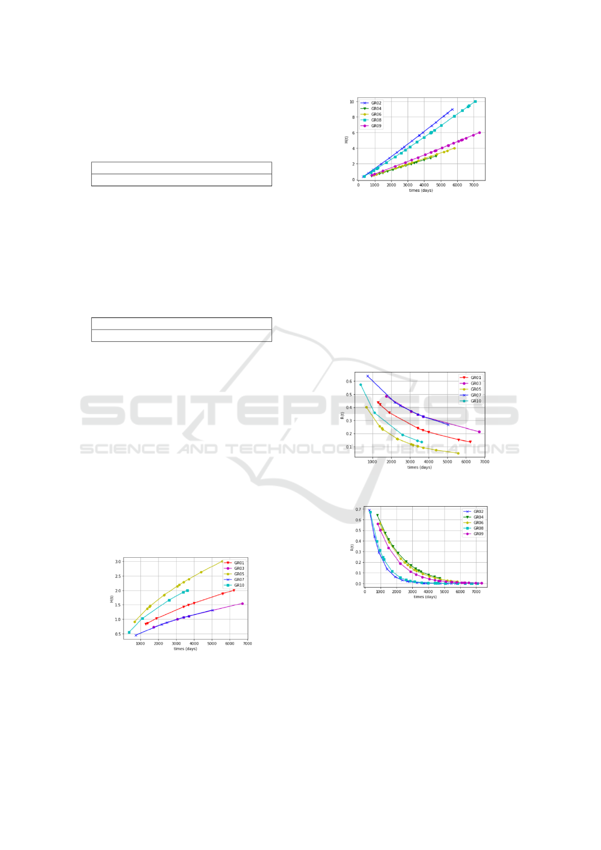
Using equation (9), we can obtain the cumulative

hazard function for GR03 and GR07 as they have no

frailty. For these groups with a non-zero frailty effect,

Equation (9) must be multiplied by the correspond-

ing z

as in Equation (3). Figures 5 and 6 illustrate

the cumulative hazard function for families A and B

respectively. In family A, GR05 is the most vulnera-

ble, representing the highest risk of cracking damage.

GR03 and GR07, on the other hand, have no frailty ef-

fect and are considered as homogeneous and more re-

liable, as shown in Figure 7. Their two curves do not

allow to conclude whether they have the same risk of

cracking or not. We can notice that they almost stick

together.

Figure 5: Cumulative Hazard function for family A.

In Figure 6, we can notice that all groups start with

the same low risk of cracking. As time goes on, the

curves become more scattered and conﬁrm the Table

8. However, the cumulative hazard function curves

Figure 6: Cumulative Hazard function for family B.

of the two groups (GR04 and GR06) stuck together.

They represent the same risk of cracking. In the same

Figure 6, curves of groups GR09, GR04 and GR06

are going in the same direction. So, instead of wasting

inspection time on both, see Table 6, the maintenance

team could decide to monitor only one of the two and

apply the same decisions obtained on the other, con-

sidering them as twin turbine runners. In the same

way, the GR02 and GR08 curves are close to each

other. An examination of the data on failure statuses

reveals that, at the end of their operating life, they

recorded multiple successive cracks.

Figure 7: Conditional reliability for A family.

Figure 8: Conditional reliability for B family.

Figures 7 and 8 have been plotted using equation

(20). They illustrate the reliability for families A and

B respectively. For the same period, 3000 days for

example, all groups in family B have a reliability be-

low 20%, whereas in family A, we have three groups

(GR01, GR03 and GR07) with a reliability above

20%. This conﬁrms that these three groups are the

most robust. The duration of systematic inspections

Reliability Analysis of Francis Turbine Cracking Using Gamma Frailty Model and Censored Historical Maintenance Data

135

could be much longer for them. Furthermore, in Fig-

ure 8, after 5,000 days, it appears that all the groups

have collapsed. These groups have been replaced or

modiﬁed supporting the model.

4 CONCLUSIONS

The study is based on a comparison of the reliabil-

ity of ten turbines belonging to two different fami-

lies, using a frailty model. To do this, we used a non-

homogeneous Poisson process with a power law and

the gamma frailty distribution. The model parameters

are found by optimizing the marginal likelihood func-

tion developed in the study. The likelihood function

takes into account censored historical maintenance

data, the gamma frailty distribution and the ﬁnal indi-

vidual observation time. In addition, the frailty effect

z is not considered as a random variable, but is de-

rived directly from the optimization of the individual

conditional likelihood function. However, for turbine

runners with no observed failures, the heterogeneity

effect was zero, which led us to abandon the frailty

model in this case. We have discovered that by de-

riving z, the frailty effect, as an expression of fail-

ure statuses and individual ﬁnal observation time, and

adding censoring to the model, the reliability curves

express the results much better and are very close to

reality. For example, groups in family B that have

been replaced due to recurring cracks have a reliabil-

ity of less than 20% at 3,000 days and have collapsed

at around 5,000 days, whereas groups in family A

are robust. Despite the fact that we neglected covari-

ates in the model, we obtained informative results that

may help the maintenance team to group turbines with

the same reliability trend and monitor only one tur-

bine in order to reduce double inspections. This study

could be strengthened by adding important covariates

such as age, turbine runner modiﬁcation, start-up and

shutdown frequencies. Future work could also focus

on optimizing systematic inspections with regard to

the evolution of reliability curves, and avoiding the

multiplication of maintenance shutdowns, which have

a negative impact on cracking.

ACKNOWLEDGEMENTS

The authors are grateful to Turbomachinery Labora-

tory of the Engineering School of the University of

Quebec in Abitibi-T

emiscamingue (UQAT), to Hydro-

ebec’s Reseach Institute and to Hydro-Qu

ebec for

the collaboration.

REFERENCES

Abbring, J. H. and Berg, G. J. V. D. (2007). The unob-

served heterogeneity distribution in duration analysis.

In Biometrika. 94(1).

Ascher, H. E. (1968). Evaluation of repairable system reli-

ability using the bad-as-old concept. In IEEE Trans-

actions on Reliability. 17(2).

Ascher, H. E. (2008). Repairable systems reliability. In

Encyclopedia of Statistics in Quality and Reliability.

Asfaw, Z. G. and Lindqvist, B. H. (2015). Unobserved het-

erogeneity in the power law nonhomogeneous poisson

process. In Reliability Engineering and System Safety.

134.

Bajgholi, M. E., Rousseau, G., Viens, M., and Thibault, D.

(2021). Capability of advanced ultrasonic inspection

technologies for hydraulic turbine runners. In pplied

Sciences. 11.

Bajgholi, M. E., Rousseau, G., Viens, M., Thibault, D., and

Gagnon, M. (2023). Reliability assessment of non de-

structive testing (ndt) for the inspection of weld joints

in the hydroelectric turbine industry. In The Interna-

tional Journal of Advanced Manufacturing Technol-

ogy. 128.

Brown, B., Liu, B., McIntyre, S., and Revie, M. (2023). Re-

liability evaluation of repairable systems considering

component heterogeneity using frailty model. In Pro-

ceedings of the Institution of Mechanical Engineers,

Part O: Journal of Risk and Reliability. 237(4).

Duchateau, L. and Janssen, P. (2008). The frailty model. In

New York: Springer Verlag. 1.

Gagnon, M. and Nicolle, J. (2019). On variations in turbine

runner dynamic behaviours observed within a given

facility. In Conference Series: Earth and Environmen-

tal Science. 450(1).

Gagnon, M., Tahan, A., Bocher, P., and Thibault, D. (2014).

Inﬂuence of load spectrum assumptions on the ex-

pected reliability of hydroelectric turbines: A case

study. In Structural Safety. 50.

Gagnon, M., Tahan, S. A., Bocher, P., and Thibault, D.

(2010). Impact of startup scheme on francis runner

life expectancy. In 25th IAHR Symposium. Timisoara.

Georgievskaia, E. (2020). Predictive analytics as a way to

smart maintenance of hydraulic turbinest. In Procedia

Structural Integrity. 28.

Georgievskaia, E. (2021). Analytical system for predicting

cracks in hydraulic turbines. In Engineering Failure

Analysis. 127.

Haji, S. H. and Abdulazeez, A. M. (2021). Comparison

of optimization techniques based on gradient descent

algorithm: A review. In PalArch’s Journal of Archae-

ology of Egyptology. 18(4).

Hydro-Qu

ebec (2023). Annual report. In Report. 1.

Ivanchenko, I. P. and Prokopenko, A. N. (2020). Analyzing

the operational materials on crack formation in blades

of francis turbines at the krasnoyarsk hpp. In . Power

Technology and Engineering. 53(6).

SIMULTECH 2024 - 14th International Conference on Simulation and Modeling Methodologies, Technologies and Applications

136

Liu, X., Luo, Y., and Wang, Z. (2016a). A review on fatigue

damage mechanism in hydro turbines. In Renewable

and Sustainable Energy Reviews. 54.

Liu, X., Luo, Y., and Wang, Z. (2016b). A review on fatigue

damage mechanism in hydro turbines. In Renewable

and Sustainable Energy Reviews. 54.

Love, C. E. and Guo, R. (1991). Application of weibull

proportional hazards modelling to bad-as-old failure

data. In Quality and reliability engineering interna-

tional. 7(3).

Morin, O., Thibault, D., and Gagnon, M. (21-26 March

2021). the comparison of hydroelectric runner fa-

tigue failure risk based on site measurements. In 30th

IAHR Symposium on Hydraulic Machinery and Sys-

tems. Lausanne.

Munda, M., Rotolo, F., and Legrand, C. (2012). parfm:

Parametric frailty models in r. In Journal of Statistical

Software. 51.

Oliveira, M. D. D., Colosimo, E. A., and Gilardoni, G. L.

(2013). Power law selection model for repairable sys-

tems. In Communications in Statistics-Theory and

Methods. 42(4).

Slimacek, V. and Lindqvist, B. H. (2016). Nonhomoge-

neous poisson process with nonparametric frailty. In

Reliability Engineering and System Safety. 149.

Therneau, T. M., Grambsch, P. M., and Pankratz, V. S.

(2003). Penalized survival models and frailty. In Jour-

nal of computational and graphical statistics. 12(1).

Thibault, D., Gagnon, M., and Godin, S. (2015). The effect

of materials properties on the reliability of hydraulic

turbine runners. In International Journal of Fluid Ma-

chinery and Systems. 8.

Trivedi, C. and Cervantes, M. (2017). Fluid-structure in-

teractions in Francis turbines : A perspective review.

Renewable and Sustainable Energy Reviews, 68, 87-

101 edition.

Trivedi, C., Gandhi, B., and Cervantes, M. (2013). ffect of

transients on francis turbine runner life: a review. In

Journal of Hydraulic Research. 51(2).

Vaupel, J. W., Manton, K. G., and Stallard, E. (2023). The

impact of heterogeneity in individual frailty on the dy-

namics of mortality. In Demography. 16(3).

Wang, X. F., Li, H. L., and Zhu, F. (2012). The calculation

of ﬂuid-structure interaction and fatigue analysis for

francis turbine runner. In IOP conference series: earth

and environmental science. 15-5.

Wienke, A. (2010). Frailty models in survival analysis. In

Chapman and Hall/CRC. 1.

Xiao, R., Wang, Z., and Luo, Y. (2008). Dynamic stresses in

a francis turbine runner based on ﬂuid-structure inter-

action analysis. In Tsinghua Science and Technology.

13(5).

Xiao, R., Wang, Z., and Luo, Y. (2010). Effect of welding

technologies on decreasing welding residual stress of

francis turbine runner. In Journal of Materials Science

and Technology. 26(10).

Zhang, Y., Zheng, X., Li, J., and Du, X. (2019). Experimen-

tal study on the vibrational performance and its phys-

ical origins of a prototype reversible pump turbine in

the pumped hydro energy storage power station. In

Renewable energy. 130.

Reliability Analysis of Francis Turbine Cracking Using Gamma Frailty Model and Censored Historical Maintenance Data

137