A Greedy Search Based Ant Colony Optimization Algorithm for

Large-Scale Semiconductor Production

Ramsha Ali

1 a

, Shahzad Qaiser

1 b

, Mohammed M. S. El-Kholany

1,3 c

, Peyman Eftekhari

1 d

Martin Gebser

1 e

, Stephan Leitner

2 f

and Gerhard Friedrich

1 g

Department of Artiﬁcial Intelligence and Cybersecurity, University of Klagenfurt, Austria

Department of Management Control and Strategic Management, University of Klagenfurt, Austria

Faculty of Computers and Artiﬁcial Intelligence, Cairo University, Egypt

Keywords:

Swarm Intelligence, Ant Colony Optimization, Greedy Search, Semiconductor Production, Scheduling.

Abstract:

This paper presents a hybrid ant colony optimization algorithm for solving large-scale scheduling problems

in semiconductor production, which can be represented as a Flexible Job Shop Scheduling Problem (FJSSP)

with the objective of minimizing the makespan required to complete all jobs. We propose a Greedy Search

based Ant Colony Optimization (GSACO) algorithm, where each ant constructs a feasible schedule using

greedy search. For the sequencing of operations, accomplished in the ﬁrst phase of GSACO, the ants adopt

a probabilistic decision rule taking pheromone trails into account. The ﬂexible machine assignment is then

greedily performed in the second phase by allocating operations one by one to an earliest available machine.

We evaluate our approach using classical FJSSP benchmarks as well as large-scale instances with about 10000

operations from the domain of semiconductor production scheduling. On these large-scale scheduling prob-

lems, our GSACO algorithm successfully overcomes the scalability limits of exact optimization by means of

a state-of-the-art Constraint Programming approach, included as baseline for our experimental comparison.

1 INTRODUCTION

Scheduling production operations in complex manu-

facturing environments is one of the most challeng-

ing resource allocation tasks. The dynamic nature of

real-world operations, subject to unpredictable pro-

cess and demand ﬂuctuations, supply chain delays,

machine breakdowns, etc., further ampliﬁes the com-

plexity. Therefore, production scheduling needs not

only be (near-)optimal, but also robust and ﬂexible to

adapt to frequent problem changes. To handle these

phenomena, a scheduling method should be efﬁcient

enough to provide and update solutions in short time.

In the scheduling literature, the Job Shop Schedul-

ing Problem (JSSP) (Xiong et al., 2022) and the Flexi-

https://orcid.org/0000-0002-4794-6560

https://orcid.org/0000-0001-6183-7638

https://orcid.org/0000-0002-1088-2081

https://orcid.org/0009-0007-4198-392X

https://orcid.org/0000-0002-8010-4752

https://orcid.org/0000-0001-6790-4651

https://orcid.org/0000-0002-1992-4049

ble Job Shop Scheduling Problem (FJSSP) (Xie et al.,

2019) stand out as popular and general scheduling

models. Both JSSP and FJSSP are NP-hard combina-

torial optimization problems, where the latter extends

JSSP by introducing ﬂexibility in assigning opera-

tions to machines. This ﬂexibility is crucial in mod-

ern manufacturing environments, as the capability to

respond to changing demands and utilize resources ef-

ﬁciently impacts the overall production performance.

In this paper, we address a large-scale Semicon-

ductor Manufacturing Scheduling Problem (SMSP)

(Kopp et al., 2020), which can also be understood as

FJSSP on instances that represent the diverse opera-

tions and high throughputs of semiconductor produc-

tion. A semiconductor manufacturing facility, called

fab for short, is a complex production environment

characterized by customized job ﬂows and high-tech

machines. Particular challenges of SMSP include:

• Long Production Routes: Hundreds of opera-

tions to be performed on a lot can span over sev-

eral months, which necessitates detailed schedul-

ing to realize an efﬁcient process ﬂow.

138

Ali, R., Qaiser, S., El-Kholany, M., Eftekhari, P., Gebser, M., Leitner, S. and Friedrich, G.

A Greedy Search Based Ant Colony Optimization Algorithm for Large-Scale Semiconductor Production.

DOI: 10.5220/0012813100003758

Paper published under CC license (CC BY-NC-ND 4.0)

In Proceedings of the 14th International Conference on Simulation and Modeling Methodologies, Technologies and Applications (SIMULTECH 2024), pages 138-149

ISBN: 978-989-758-708-5; ISSN: 2184-2841

• Product-Speciﬁc Machine Setups: Production

operations may require speciﬁc machine setups,

which increases the complexity of operation se-

quencing and machine allocation.

• Maintenance and Stochastic Events: Preven-

tive maintenance procedures and unpredictable

yet frequent events, such as machine breakdowns

or process deviations, demand for a highly adap-

tive and responsive scheduling system.

To meet the growing demands for semiconductors

and manage the complexity of modern semiconduc-

tor production, manufacturers are increasingly striv-

ing for automated production scheduling and control

systems. Such systems are conceived to optimize the

resource utilization, regulate sophisticated sequences

of manufacturing steps, and adjust to process devia-

tions in real time. The overall goal is to minimize

the production times and costs, while maximizing fab

throughput and product quality.

In contrast to classical FJSSP benchmarks, where

small to medium-scale instances include up to 500 op-

erations and 60 machines (Behnke and Geiger, 2012),

modern semiconductor fabs process tens of thousands

of operations per day using more than 1000 machines

(Kopp et al., 2020). These machines are organized in

tool groups with speciﬁc functionalities, e.g., diffu-

sion, etching, or metrology, and each manufacturing

step can be ﬂexibly allocated to a machine providing

the required functionality. Hence, the scheduling of

semiconductor production operations consists of the

sub-tasks of assigning operations to machines and se-

quencing the operations on each machine. However,

in case of machine breakdowns or process deviations,

a schedule must be revised to adapt to the changed en-

vironment. To this end, we propose a Greedy Search

based Ant Colony Optimization (GSACO) algorithm

for (re-)scheduling semiconductor production oper-

ations. Our algorithm harnesses Ant Colony Opti-

mization (ACO) (Dorigo and St

utzle, 2019) for ex-

ploration, while Greedy Search (GS) (Papadimitriou

and Steiglitz, 1982) enables responses in short time.

In this way, GSACO overcomes limitations of a state-

of-the-art Constraint Programming approach (Perron

et al., 2023) on large-scale SMSP instances.

The paper is organized as follows. Section 2 pro-

vides literature reviews on FJSSP and ACO. In Sec-

tion 3, we formulate SMSP in terms of the well-

known FJSSP. Our GSACO algorithm is presented in

Section 4. Section 5 provides and discusses experi-

mental results. Finally, Section 6 concludes the paper.

2 LITERATURE REVIEW

We brieﬂy survey the relevant literature on FJSSP,

which we use as general scheduling model to repre-

sent semiconductor production processes and SMSP,

as well as ACO and its application to FJSSP solving.

2.1 Flexible Job Shop Scheduling

Exact mathematical models of the NP-hard FJSSP

allow for solving small-scale instances to optimal-

ity. For example, (Meng et al., 2020) devise Mixed-

Integer Linear Programming (MILP) and Constraint

Programming (CP) models for a distributed FJSSP

setting. They observe that CP performs well at ex-

ploring feasible solutions, leading to high-quality so-

lutions in relatively short computing time. Similarly,

(Gedik et al., 2018) make use of a CP model to effec-

tively solve small to medium-scale FJSSP instances.

The scalability limits of exact optimization ap-

proaches motivate the design of approximation meth-

ods, where a large variety of heuristics and meta-

heuristics have been proposed for FJSSP solving.

Respective techniques include tabu search (Saidi-

Mehrabad and Fattahi, 2007), simulated annealing

(Sobeyko and M

onch, 2016), particle swarm opti-

mization (Gao et al., 2006), genetic algorithms (Ho

et al., 2007), artiﬁcial bee colony algorithms (Li et al.,

2014), and ACO (Wang et al., 2017) as well as hybrid

approaches based on local search with meta-heuristics

(Li et al., 2010; Xing et al., 2010; Thammano and

Phu-ang, 2013; El Khoukhi et al., 2017).

In their recent work, (Shang, 2023) train deep neu-

ral networks on historical FJSSP data to identify pat-

terns and predict effective scheduling strategies. Re-

lated approaches based on deep reinforcement learn-

ing (St

ockermann et al., 2023; Tassel et al., 2023) or

genetic algorithms (Kov

acs et al., 2023) aim at opti-

mizing the decision making and control within sim-

ulation models of semiconductor fabs. While these

methods allocate production lots one by one based on

their features, we address the task of scheduling the

operations on given lots in advance.

2.2 Ant Colony Optimization

ACO is a meta-heuristic algorithm that mimics the

foraging behavior of ants (Dorigo and St

utzle, 2019).

It was originally devised to solve the traveling sales-

person problem (St

utzle and Dorigo, 1999), and

meanwhile ACO has been adopted to various opti-

mization problems, including routing (Rizzoli et al.,

2007), scheduling (Luo et al., 2008), task allocation

(Rugwiro et al., 2019), project planning (Khelifa and

A Greedy Search Based Ant Colony Optimization Algorithm for Large-Scale Semiconductor Production

139

Table 1: Basic notations.

Symbol Description

J Total number of jobs

T Total number of tool groups

M Total number of machines

N Total number of operations

Tool group t of machine m

i, j,t

Operation i of job j on tool group t

i, j,t

Duration of operation O

i, j,t

on tool group t

i, j,t,m

Operation i of job j on machine m of tool group t

i, j,t,m

Start time of operation O

i, j,t

on machine m of tool group t

Laouar, 2020), and network optimization (Wang et al.,

2009).

The common idea is that artiﬁcial ants construct

paths through a graph, making probabilistic deci-

sions based on problem-speciﬁc heuristic information

as well as temporary pheromone trails that indicate

promising search directions. Particular strengths of

ACO lie in the high potential for parallelization, given

that ants can be simulated in parallel, and a certain

robustness against getting stuck in local optima, as

the probabilistic decision rules of ants promote explo-

ration. However, a speciﬁc difﬁculty in the ACO algo-

rithm design concerns the tuning of hyperparameters,

such as the number of ants to consider, the trade-off

between heuristic information and pheromone trails,

and the pheromone evaporation rate.

Among meta-heuristic FJSSP solving techniques,

ACO has been shown to be a particularly promising

approach (T

urkyılmaz et al., 2020). The practical dif-

ﬁculty remains to escape local optima and reliably

converge to high-quality solutions within a short com-

puting time limit. This challenge has brought about a

variety of extended ACO algorithms as well as hy-

brid approaches that combine ACO with local search

methods (Leung et al., 2010; Li et al., 2010; Xing

et al., 2010; Thammano and Phu-ang, 2013; Arnaout

et al., 2014; El Khoukhi et al., 2017). While these

methods have been designed and evaluated on small

to medium-scale FJSSP benchmarks (Arnaout et al.,

2014), our work addresses the large-scale SMSP in-

stances encountered in the domain of semiconduc-

tor production scheduling (Kopp et al., 2020). Be-

yond FJSSP and SMSP investigated here, we note

that hybrid optimization algorithms integrating meta-

heuristics and local search have also been adopted in

a variety of other application settings (Abdel-Basset

et al., 2021; Fontes et al., 2023; Li et al., 2021;

Mohd Tumari et al., 2023; Suid and Ahmad, 2023).

3 PROBLEM FORMULATION

We formulate SMSP in terms of the general FJSSP

model, using the basic notations listed in Table 1. In

detail, our setting for scheduling the production of a

semiconductor fab is characterized as follows:

• The fab consists of M machines, which are parti-

tioned into T tool groups, where t

∈ {1, . . . , T }

denotes the tool group to which a machine m ∈

{1, . . . , M} belongs.

• There are J jobs, where each j ∈ {1, . . . , J} repre-

sents a sequence O

1, j,t

, . . . , O

, j,t

of operations

to be performed on a production lot. Note that

∈ {1, . . . , T } speciﬁes the tool group responsi-

ble for processing an operation O

i, j,t

, but not a

speciﬁc machine of t

, which reﬂects ﬂexibility in

assigning operations to machines. The total num-

ber of operations is denoted by N =

∑

j∈{1,...,J}

• For each operation O

i, j,t

, the duration d

i, j,t

is re-

quired for processing O

i, j,t

on some machine of

the tool group t.

Our SMSP model reﬂects several features orig-

inating from the semiconductor production scenar-

ios of the SMT2020 dataset (Kopp et al., 2020). In

the SMT2020 scenarios, jobs are associated with par-

ticular products, and their operation sequences, also

called production routes, coincide for the same prod-

uct. Since such production routes include hundreds of

operations that are performed over several months in

the physical fab, distinct lots of the same product are

frequently at different steps of their routes when they

get (re-)scheduled. Hence, we do not explicitly dis-

tinguish production routes by products but consider

operation sequences of length n

relative to a job j,

which allows for separating the operations on lots that

are at different manufacturing steps of the same route.

Moreover, the machines belonging to a tool group

are assumed to be uniform, i.e., an operation requir-

ing the tool group can be processed by any of its ma-

SIMULTECH 2024 - 14th International Conference on Simulation and Modeling Methodologies, Technologies and Applications

140

Table 2: GSACO parameters.

Parameter Description

l Cycles/time limit

n Planning horizon

k Number of ants

Initial pheromone level

Minimum pheromone level

Pheromone level on edge e

ρ Evaporation rate

c Contribution of best schedules

chines. This simplifying assumption ignores speciﬁc

machine setups, which may be needed for some op-

erations and take additional equipping time, as well

as unavailabilities due to maintenance procedures or

breakdowns. However, the greedy machine assign-

ment performed by our GSACO algorithm in Sec-

tion 4 can take such conditions into account for allo-

cating an operation to the earliest available machine.

In addition, some transportation time is required to

move a lot from one machine to another between op-

erations, which is not explicitly given but taken as part

of the operation duration in the SMT2020 scenarios.

A schedule allocates each operation O

i, j,t

to some

machine m ∈ {1, . . . , M} such that t

= t, and we de-

note the machine assignment by O

i, j,t,m

. Each ma-

chine performs its assigned operations in sequence

without preemption, i.e., s

i, j,t,m

+ d

i, j,t

≤ s

′

, j

′

,t,m

′

, j

′

,t,m

+ d

′

, j

′

≤ s

i, j,t,m

must hold for the start times

i, j,t,m

and s

′

, j

′

,t,m

of operations O

i, j,t,m

̸= O

′

, j

′

,t,m

al-

located to the same machine m. The precedence be-

tween operations of a job j ∈ {1, . . . , J} needs to be

respected as well, necessitating that s

i, j,t,m

+ d

i, j,t

≤

i+1, j,t

′

when i < n

. Assuming that 0 ≤ s

1, j,t,m

for

each job j ∈ {1, . . . , J}, the makespan to complete all

jobs is given by max{s

, j,t,m

, j,t

| j ∈ {1, . . . , J}}.

We take makespan minimization as the optimization

objective for scheduling, since it reﬂects efﬁcient ma-

chine utilization and maximization of fab throughput.

An example schedule (generated by GSACO) for

three jobs with three operations each is displayed in

Figure 5. The start times for the operations of job 1

illustrate the scheduling constraints. That is, we have

1,1,3,5

+ d

1,1,3

= 0 + 10 = s

2,1,4,7

due to the prece-

dence between the ﬁrst and second operation, while

the machine 7 performing the second operation is

already available at time 9. Regarding the start of

the third operation, s

2,1,4,7

+ d

2,1,4

= 10 + 2 < 13 =

3,1,1,1

, i.e., the third operation needs to wait for ma-

chine 1 to complete the execution of another opera-

tion (of job 2). The completion time s

3,3,1,2

+ d

3,3,1

12 + 13 of the third operation of job 3 constitutes the

makespan 25 of the example schedule in Figure 5.

Input: dataset, l

Output: best schedule found by ants

Parameters: n, k, τ

, τ

, ρ, c

Initialize adjacency, pheromone, and machine

matrix;

makespan ← ∞;

while cycle or time limit l is not reached do

foreach ant from 1 to k do

Run GS procedure to ﬁnd a schedule;

end

new ← shortest makespan of ants’ schedules;

if new < makespan then

makespan ← new;

best ← an ant’s schedule of makespan;

end

foreach edge e in pheromone matrix do

← max{ρ · τ

, τ

}; // evaporation

end

foreach edge e selected by best ant do

← τ

+ c; // deposit pheromones

end

return best;

Algorithm 1: Greedy Search based ACO (GSACO).

4 GSACO ALGORITHM

The framework of our GSACO algorithm, whose (in-

put and internal) parameters are summarized in Ta-

ble 2, is displayed in Figure 1. Its four submodules,

indicated in bold, are described in separate subsec-

tions below.

Moreover, Algorithm 1 provides a pseudo-code

representation of GSACO. For a conﬁgurable cycle

number or time limit l, each of the k ants applies

greedy search using the GS procedure (detailed in Al-

gorithm 2). That is, the ﬁrst GS phase constructs an

operation sequence, which is then taken as basis for

greedily assigning the operations to machines in the

second phase. Note that the ants run independently,

so that their GS trials can be performed in parallel.

As a result, k schedules along with edges between op-

erations (described in Subsection 4.2) that have been

selected for their construction are obtained. If some

of these schedules improves the makespan over the

best schedule found in previous iterations (if any), the

best schedule gets updated. As common for ACO al-

gorithms, pheromones τ

on edges e are subject to

evaporation, according to the formula ρ · τ

, while

edges selected to construct the best schedule obtained

so far also receive a pheromone contribution, calcu-

lated as τ

+ c. Such pheromone deposition increases

the chance for edges contributing to the current best

A Greedy Search Based Ant Colony Optimization Algorithm for Large-Scale Semiconductor Production

141

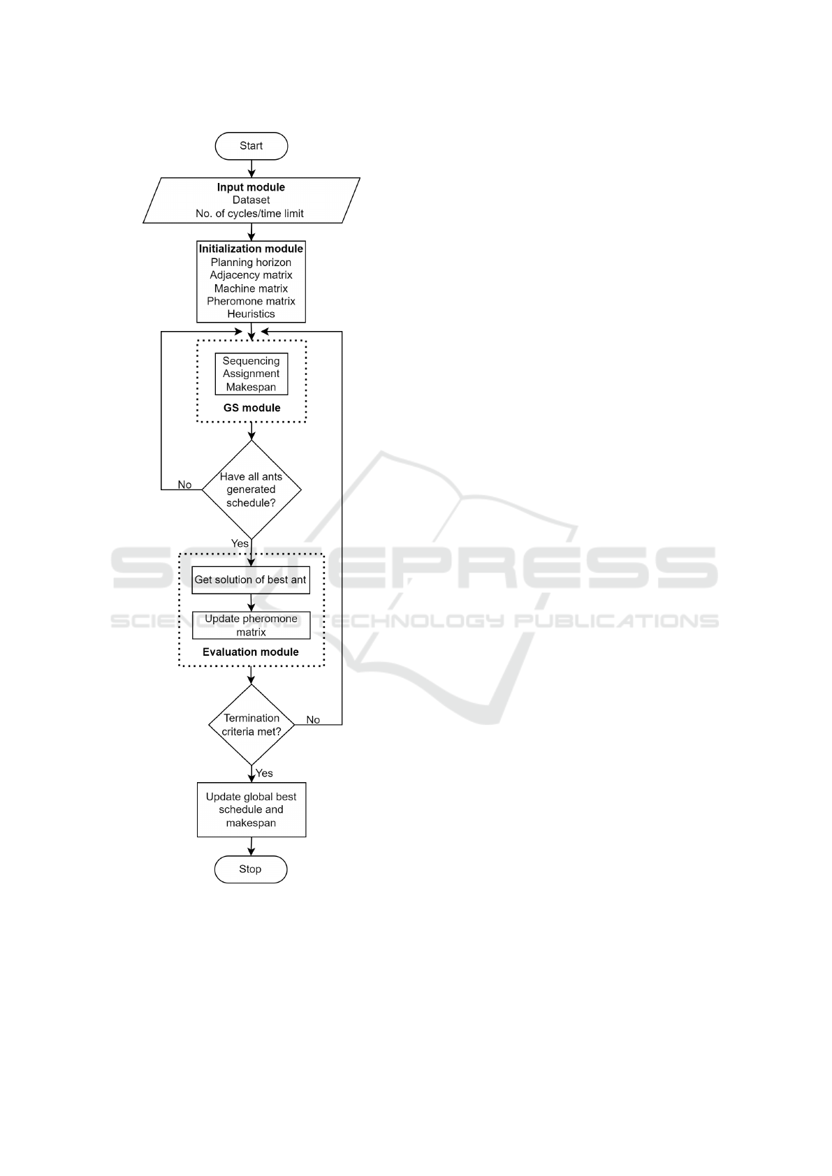
Figure 1: GSACO framework.

schedule to get re-selected in forthcoming iterations.

4.1 Input Module

This module reads in an SMSP instance, e.g., ob-

tained from the SMT2020 dataset (Kopp et al., 2020),

specifying production routes, the tool groups with

their machines, and the jobs to be performed. More-

over, a limit l on the number of cycles and/or the time

to spend on optimization by GSACO is given as input.

4.2 Initialization Module

In view of long production routes with hundreds of

operations in the SMT2020 dataset, we introduce a

conﬁgurable planning horizon n as upper bound on

the length n

of the operation sequence for a job j.

The planning horizon thus constitutes a scaling factor

for the size and the resulting complexity of SMSP in-

stances. In practice, unpredictable stochastic events

make long-term schedules obsolete and necessitate

frequent re-scheduling, where limiting the planning

horizon upfront provides a means to control the search

and enable short response times.

To express SMSP as a search problem on graphs,

we identify an instance with the disjunctive graph G =

(V, E

∪ E

), whose vertices V contain the operations

i, j,t

plus a dummy start node 0, conjunctive edges

= {(0, O

1, j,t

) | O

1, j,t

∈ V }

∪ {(O

i−1, j,t

i−1

, O

i, j,t

) | O

i, j,t

∈ V, i > 1}

connect the dummy start node 0 to the ﬁrst operation

and each operation on to its successor (if any) in the

sequence for a job, and disjunctive edges

= {(O

i, j,t

, O

′

, j

′

) | O

i, j,t

∈ V, O

′

, j

′

∈ V, j ̸= j

′

}

link operations (of distinct jobs) sharing a common

tool group, as such operations may be allocated to

the same machine. Any feasible schedule induces an

acyclic subgraph (V, E) of the disjunctive graph G

such that E

⊆ E, and (O

i, j,t

, O

′

, j

′

) ∈ E

∩ E iff

i, j,t,m

+ d

i, j,t

< s

′

, j

′

,t,m

for distinct jobs j ̸= j

′

, i.e.,

the operation O

i, j,t

is processed before O

′

, j

′

by the

same machine m of tool group t

= t. Conversely,

the search for a high-quality solution can be accom-

plished by determining an acyclic subgraph (V, E)

of G that represents a schedule of short makespan.

For example, Table 3 shows nine operations be-

longing to the operation sequences for three jobs, as

they can be obtained with the parameter n = 3 for

the planning horizon. Conjunctive edges connect the

dummy start node 0 to the operations numbered 1, 4,

and 7, which come ﬁrst in their jobs, then operation 1

is connected on to 2 as well as 2 to 3, and similarly

for the other two jobs. In addition, mutual disjunc-

tive edges link operations to be processed on the same

SIMULTECH 2024 - 14th International Conference on Simulation and Modeling Methodologies, Technologies and Applications

142

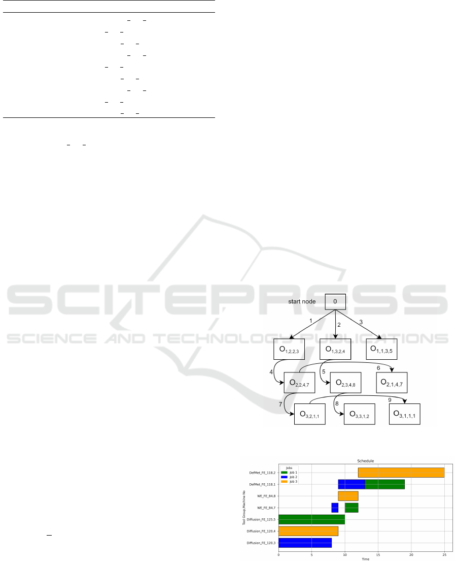
Table 3: Example operations.

No. Operation Tool group name Duration

1 O

1,1,3

Diffusion FE 125 10

2 O

2,1,4

WE FE 84 2

3 O

3,1,1

DefMet FE 118 6

4 O

1,2,2

Diffusion FE 120 8

5 O

2,2,4

WE FE 84 1

6 O

3,2,1

DefMet FE 118 4

7 O

1,3,2

Diffusion FE 120 9

8 O

2,3,4

WE FE 84 3

9 O

3,3,1

DefMet FE 118 13

tool group, e.g., those numbered 4 and 7 have the tool

group Diffusion FE 120 in common. The resulting

(N + 1) × (N + 1) adjacency matrix, where N = 9 is

the total number of operations, 0 entries indicate the

absence, and 1 entries the existence of edges, is given

in Figure 2.

0 1 2 3 4 5 6 7 8 9







0 1 0 0 1 0 0 1 0 0

0 0 1 0 0 0 0 0 0 0

0 0 0 1 0 1 0 0 1 0

0 0 0 0 0 0 1 0 0 1

0 0 0 0 0 1 0 1 0 0

0 0 1 0 0 0 1 0 1 0

0 0 0 1 0 0 0 0 0 1

0 0 0 0 1 0 0 0 1 0

0 0 1 0 0 1 0 0 0 1

0 0 0 1 0 0 1 0 0 0







Figure 2: Adjacency matrix for the operations in Table 3.

As initial pheromone level on edges e ∈ E

∪ E

we take τ

= 1 by default. In general, representing

pheromone levels by an (N +1)×(N +1) matrix sim-

ilar to the adjacency matrix, the entries τ

are initial-

ized according to the following condition:

(

if e ∈ E

∪ E

0 otherwise

With τ

= 1, this reproduces the adjacency matrix in

Figure 2 as initial pheromone matrix for our example.

We additionally represent the possible machine

assignments by an (N + 1) × M machine matrix,

where M is the total number of machines. For exam-

ple, with two machines per tool group and the map-

ping t

= ⌈

⌉ from machine identiﬁers m ∈ {1, . . . , 8}

to the tool groups t ∈ {1, . . . , 4}, responsible for pro-

cessing the operations in Table 3, we obtain the ma-

chine matrix shown in Figure 3. While the dummy

start node 0 needs no machine to process it, the oper-

ation O

1,1,3

numbered 1 can be allocated to either the

machine 5 or 6 of tool group 3, and corresponding 1

entries indicate the machines available to perform the

other operations as well.

1 2 3 4 5 6 7 8







0 0 0 0 0 0 0 0

0 0 0 0 1 1 0 0

0 0 0 0 0 0 1 1

1 1 0 0 0 0 0 0

0 0 1 1 0 0 0 0

0 0 0 0 0 0 1 1

1 1 0 0 0 0 0 0

0 0 1 1 0 0 0 0

0 0 0 0 0 0 1 1

1 1 0 0 0 0 0 0







Figure 3: Machine matrix for the operations in Table 3.

4.3 GS Module

The general goal of greedy search methods consists of

using heuristic decisions to ﬁnd high-quality, but not

necessarily optimal solutions in short time. Within

GSACO, each ant applies greedy search to efﬁciently

construct some feasible schedule for a given SMSP

instance. The respective GS procedure, outlined by

the pseudo-code in Algorithm 2, includes two phases:

operation sequencing and machine assignment.

Figure 4: Example run of GS procedure.

Figure 5: Feasible schedule for the operations in Table 3.

The ﬁrst phase constructs a sequence comprising

all operations of an SMSP instance. To this end, a

probabilistic decision rule based on the pheromone

A Greedy Search Based Ant Colony Optimization Algorithm for Large-Scale Semiconductor Production

143

Output: schedule and selected edges of an ant

sequence ← [];

selected ←

next ← {(0, O

1, j,t

) | j ∈ {1, . . . , J}};

while next ̸=

0 do

foreach e ∈ next do p

←

∑

′

∈next

′

;

Randomly select an edge e based on p

;

for selected edge e = (O

′

, O

i, j,t

) do

sequence.enqueue(O

i, j,t

);

selected ← selected ∪ {e};

next ← {(O

, O

) ∈ next | O

̸= O

i, j,t

};

E ← {(O

i, j,t

, O

i+1, j,t

′

) | i < n

}

∪ {(O

i, j,t

, O

′

, j

′

) | (O

, O

′

, j

′

) ∈ next};

next ← next ∪ E;

end

foreach m ∈ {1, . . . , M} do a

← 0;

while sequence ̸= [] do

i, j,t

← sequence.dequeue();

a ← ∞;

foreach m from 1 to to M do

if t

= t and a

< a then

a ← a

;

b ← m;

end

i, j,t,b

← max({a}

∪ {s

i−1, j,t

′

+ d

i−1, j,t

′

| i > 1});

← s

i, j,t,b

+ d

i, j,t

;

end

return ⟨{s

i, j,t,m

| (O

′

, O

i, j,t

) ∈ selected}, selected⟩;

Algorithm 2: Greedy Search (GS).

matrix selects edges (O

′

, O

i, j,t

) and adds their target

operations O

i, j,t

to the sequence one by one. As in-

variant ensuring the feasibility of a resulting schedule,

the predecessor operation O

i−1, j,t

′

of the same job j

must already belong to the sequence in case i > 1.

This is accomplished by maintaining a set next of se-

lectable conjunctive and disjunctive edges (O

′

, O

i, j,t

)

such that O

′

is the dummy start node 0 or already in

sequence, while O

i, j,t

is the ﬁrst yet unsequenced op-

eration of its job j.

For example, starting with an empty sequence for

the operations in Table 3, the initially selectable edges

are (0, O

1,1,3

), (0, O

1,2,2

), and (0, O

1,3,2

). Assuming

that (0, O

1,2,2

) gets selected, the ﬁrst operation O

1,2,2

of job 2 is added to the sequence, and the conjunc-

tive edge (O

1,2,2

, O

2,2,4

) as well as the disjunctive

edge (O

1,2,2

, O

1,3,2

) replace (0, O

1,2,2

) among the se-

lectable edges. The process of selecting some edge

to a yet unsequenced operation is repeated until each

operation along with an edge targeting it has been pro-

cessed. Note that selected disjunctive edges link oper-

ations based on tool groups, i.e., they do not reﬂect a

machine assignment to be made in the second phase.

With a sequence of operations at hand, the sec-

ond phase allocates operations one by one to an ear-

liest available machine. Reconsidering the operations

1,2,2

and O

1,3,2

as well as the machine matrix in Fig-

ure 3, where these operations are numbered 4 and 7,

we can ﬁrst allocate O

1,2,2

to the free machine 3 with

the start time s

1,2,2,3

= 0. This means that machine 3

becomes available again at time a

= s

1,2,2,3

1,2,2

8. However, the other machine 4 of tool group 2 is

still free, so that O

1,3,2

is greedily assigned to ma-

chine 4 with the start time s

1,3,2,4

= 0 and the updated

availability a

= s

1,3,2,4

+ d

1,3,2

= 9. As we have that

= 8 < 9 = a

, if a third operation were to be al-

located to either the machine 3 or 4 of tool group 2,

our greedy assignment strategy would decide for ma-

chine 3. The described machine assignment process

allocates operations according to the sequence from

the ﬁrst phase, yielding a feasible schedule that as-

signs the machines and start times for all operations.

Figure 4 displays a sequence for the operations in

Table 3, where sequence numbers indicate the order

in which edges to the operations are selected, as it

can be generated by the GS procedure. The edges

running vertically are conjunctive and connect the

dummy start node 0 to the ﬁrst operations of the three

jobs as well as predecessors to their successor opera-

tions. In addition, two disjunctive edges are selected

between the second or third operation, respectively, of

job 2 and the corresponding operation of job 1, con-

sidering that these operations have the tool group 4

or 1 in common.

The resulting greedy machine assignment, com-

puted in the second phase of the GS procedure, is de-

noted by m within the node labels O

i, j,t,m

in Figure 4.

In view of two machines available per tool group and

three operations sharing each of the tool groups 1

and 4, the ﬁrst two operations according to the se-

quence from the ﬁrst phase, i.e., O

2,2,4

and O

2,3,4

3,2,1

and O

3,3,1

, respectively, get distributed among

the two machines of each tool group, which leads to

the machine assignments O

2,2,4,7

and O

2,3,4,8

as well

as O

3,2,1,1

and O

3,3,1,2

. Which machines of the tool

groups 4 and 1 then become available ﬁrst to allocate

the operations O

2,1,4

and O

3,1,1

can be read off the cor-

responding schedule shown in Figure 5. That is, the

machine 7 of tool group 4 is available from time 9,

yielding the greedy assignment O

2,1,4,7

. Similarly,

3,1,1,1

is obtained because the machine 1 gets free

at time 13, while the other machine 2 of tool group 1

processes the third operation of job 3 until time 25,

which is the makespan of the constructed schedule.

SIMULTECH 2024 - 14th International Conference on Simulation and Modeling Methodologies, Technologies and Applications

144

0 1 2 3 4 5 6 7 8 9







0 1.3 0 0 1.3 0 0 1.3 0 0

0 0 1.3 0 0 0 0 0 0 0

0 0 0 1.3 0 4.9 0 0 4.9 0

0 0 0 0 0 0 4.9 0 0 4.9

0 0 0 0 0 1.3 0 4.9 0 0

0 0 4.9 0 0 0 1.3 0 4.9 0

0 0 0 4.9 0 0 0 0 0 4.9

0 0 0 0 4.9 0 0 0 1.3 0

0 0 4.9 0 0 4.9 0 0 0 1.3

0 0 0 4.9 0 0 4.9 0 0 0







Figure 6: Updated pheromone matrix for the operations in Table 3 after a few GSACO iterations.

Given that this makespan coincides with the cumula-

tive duration of job 3 and its operations must be pro-

cessed in sequence, the feasible schedule in Figure 5

happens to be optimal for the operations in Table 3.

4.4 Evaluation Module

While each ant independently constructs a feasible

schedule by means of the GS procedure, the evalu-

ation module collects the results obtained by the ants

in a GSACO iteration. Among them, a schedule of

shortest makespan is determined as outcome of the

iteration and stored as new best solution in case it im-

proves over the schedules found in previous iterations

(if any). After evaporating pheromones τ

by ρ · τ

where τ

remains as minimum pheromone level if the

obtained value would be smaller, the edges e that have

been selected by the GS procedure for constructing

the current best schedule receive a pheromone contri-

bution and are updated to τ

+ c.

Note that our contribution parameter c is a

constant, while approaches in the literature often

take the inverse of an objective value (T

urkyılmaz

et al., 2020), i.e., of the makespan in our case.

The latter requires careful scaling to obtain non-

marginal pheromone contributions, in particular,

when makespans get as large as for SMSP instances.

We instead opt for pheromone contributions such that

the edges selected to construct best schedules are cer-

tain to have an increased chance of getting re-selected

in forthcoming iterations. For our example in Table 3,

Figure 6 provides the updated pheromone matrix after

a few iterations of GSACO with the parameter values

ρ = 0.7 and c = 0.5, showing a clear separation be-

tween the more frequently selected and futile edges.

5 EXPERIMENTAL EVALUATION

We implemented our GSACO algorithm in Python us-

ing PyTorch, as it handles tensor operations efﬁciently

Table 4: GSACO input parameter values.

Parameter Value

l 10

n 1–5

k 10

0.00001

ρ 0.7

c 0.5

and provides a multiprocessing library for paralleliza-

tion, thus signiﬁcantly speeding up the ants’ execution

of the GS procedure in each GSACO iteration.

The

ﬁrst challenge consists of determining suitable val-

ues for the input parameters listed in Table 2, i.e., all

parameters but the internally calculated pheromone

level τ

on edges e. We commit to the values given

in Table 4, where a time limit l of 10 minutes and a

planning horizon n of up to 5 operations per job are

plausible for SMSP instances based on the SMT2020

dataset, whose stochastic events necessitate frequent

re-scheduling in practice. For the initial pheromone

level τ

, we start from value 1, and take 0.00001 as

the minimum τ

to avoid going down to 0, consider-

ing that the GS procedure can only select edges with

non-zero entries in the pheromone matrix. The val-

ues for the number k of ants, the evaporation rate ρ,

and the pheromone contribution c are more sophisti-

cated to pick. That is, we tuned these parameters in a

trial-and-error process that, starting from a baseline,

inspects deviations of the ﬁnal makespan and con-

vergence speed obtained with iterative modiﬁcations.

Certainly, an automated approach would be desirable

to perform this task efﬁciently for new instance sets.

To compare GSACO with the state of the art in

FJSSP solving, we also run the CP solver OR-Tools

(version 9.5) (Perron et al., 2023), while heuristic

and meta-heuristic methods from the literature could

not be reproduced due to the inaccessibility of source

The source code is publicly available in our GitHub

repository: https://github.com/prosysscience/GSACO

A Greedy Search Based Ant Colony Optimization Algorithm for Large-Scale Semiconductor Production

145

Table 5: FJSSP results obtained with CP and GSACO.

Instance J M CP GSACO

MK1 10 6 40 44

MK2 10 6 27 40

MK3 15 8 204 239

MK4 15 8 60 83

SFJSSP1 2 2 66 66

SFJSSP2 2 2 107 107

SFJSSP3 3 2 221 221

SFJSSP4 3 2 355 355

MFJSSP1 5 6 468 498

MFJSSP2 5 7 446 470

MFJSSP3 6 7 466 523

MFJSSP4 7 7 554 664

code or tuned hyperparameters. Note that CP ap-

proaches have been shown to be particularly effec-

tive among exact optimization techniques for FJSSP

(Ku and Beck, 2016), where the free and open-source

solver OR-Tools excels as serial winner of the Mini-

Zinc Challenge.

We performed our experiments on

a TUXEDO Pulse 14 Gen1 machine equipped with

an 8-core AMD Ryzen 7 4800H processor at 2.9GHz

and onboard Radeon graphics card.

Table 5 illustrates the strengths of CP models on a

benchmark set of small to medium-scale FJSSP in-

stances (Arnaout et al., 2014), where the instances

MK1–MK4 are due to (Brandimarte, 1993) and the

remaining eight instances have been introduced in

(Fattahi et al., 2007). In view of the small numbers J

and M of jobs or machines, respectively, in these clas-

sical FJSSP instances, OR-Tools solves all of them to

optimality within a few seconds, so that the CP col-

umn shows the minimal makespan for each instance.

Since GSACO is an approximation method, its best

schedules are not necessarily optimal, as it can be

observed on instances other than SFJSSP1–SFJSSP4.

This reconﬁrms that exact models, particularly those

based on CP (Ku and Beck, 2016), are the ﬁrst choice

for FJSSP instances of moderate size and complexity.

To evaluate large-scale SMSP instances, we con-

sider two semiconductor production scenarios of the

SMT2020 dataset: Low-Volume/High-Mix (LV/HM)

and High-Volume/Low-Mix (HV/LM). As indicated

in Table 6, both scenarios include more than 2000

jobs and more than 1300 machines, modeling the

production processes of modern semiconductor fabs.

The main difference is given by the number of

products and associated production routes for jobs,

where LV/HM considers 10 production routes vary-

ing between 200–600 steps in total, while HV/LM

comprises 2 production routes with about 300 or

600 steps, respectively. Originally, the LV/HM and

https://www.minizinc.org/challenge

Table 6: Number of jobs, machines, and operations for

SMSP instances.

Scenario J M O

LV/HM 2156 1313 up to 10747

HV/LM 2256 1443 up to 11218

HV/LM scenarios have been designed to represent fab

load at the start of simulation runs, so that the jobs

are at different steps of their production routes. We

here instead focus on scheduling for planning hori-

zons n from 1 to 5, standing for the up to 5 next oper-

ations to be performed per job. Hence, the operations

O to schedule gradually increase from the number J

of jobs, in case of the planning horizon n = 1, to more

than 10000 operations for the longest horizon n = 5.

While running with a time limit l of 10 min-

utes, Table 7 reports the makespans of current best

schedules found by the CP solver OR-Tools and our

GSACO implementation at 1, 3, 5, 7, and 9 minutes

of computing time. Considering that the SMSP in-

stances are large, OR-Tools now takes 3 minutes to

come up with the ﬁrst solution(s) for the shortest plan-

ning horizon n = 1 on the LV/HM scenario. Within

the same fraction of computing time, GSACO already

converges to a makespan of 3725 and then proceeds

with iterations that do not yield further improvements.

That the best schedule found by GSACO is not opti-

mal is witnessed by a marginally better solution ob-

tained by OR-Tools after 7 minutes. However, for the

other SMSP instances, OR-Tools is unable to improve

over GSACO within 9 minutes, and it cannot even

provide feasible schedules for planning horizons from

n = 2 on the HV/LM scenario or n = 3 on LV/HM.

The quick convergence of our GSACO imple-

mentation is also outlined by the makespan improve-

ments plotted in Figure 7. On the LV/HM scenario

displayed in Figure 7(a), GSACO obtains its best

schedules within 7 minutes for all planning horizons.

Only for the longest planning horizon n = 5 on the

HV/LM scenario in Figure 7(b), an improvement oc-

curs after more than the 9 minutes of computing time

listed in the rightmost column of Table 7. Compar-

ing the SMSP instances for which OR-Tools man-

ages to provide feasible schedules, the convergence

to makespans in roughly the range of GSACO’s re-

sults takes signiﬁcantly more computing time. Hence,

the time limit that would be necessary to break even

with GSACO, as accomplished within 7 minutes for

the shortest planning horizon n = 1 on the LV/HM

scenario, cannot be predicted for the SMSP instances

with longer planning horizons. Moreover, we observe

that the initial schedules obtained in the ﬁrst GSACO

iteration by some of the ants running in parallel are

of relatively high quality, while OR-Tools sometimes

SIMULTECH 2024 - 14th International Conference on Simulation and Modeling Methodologies, Technologies and Applications

146

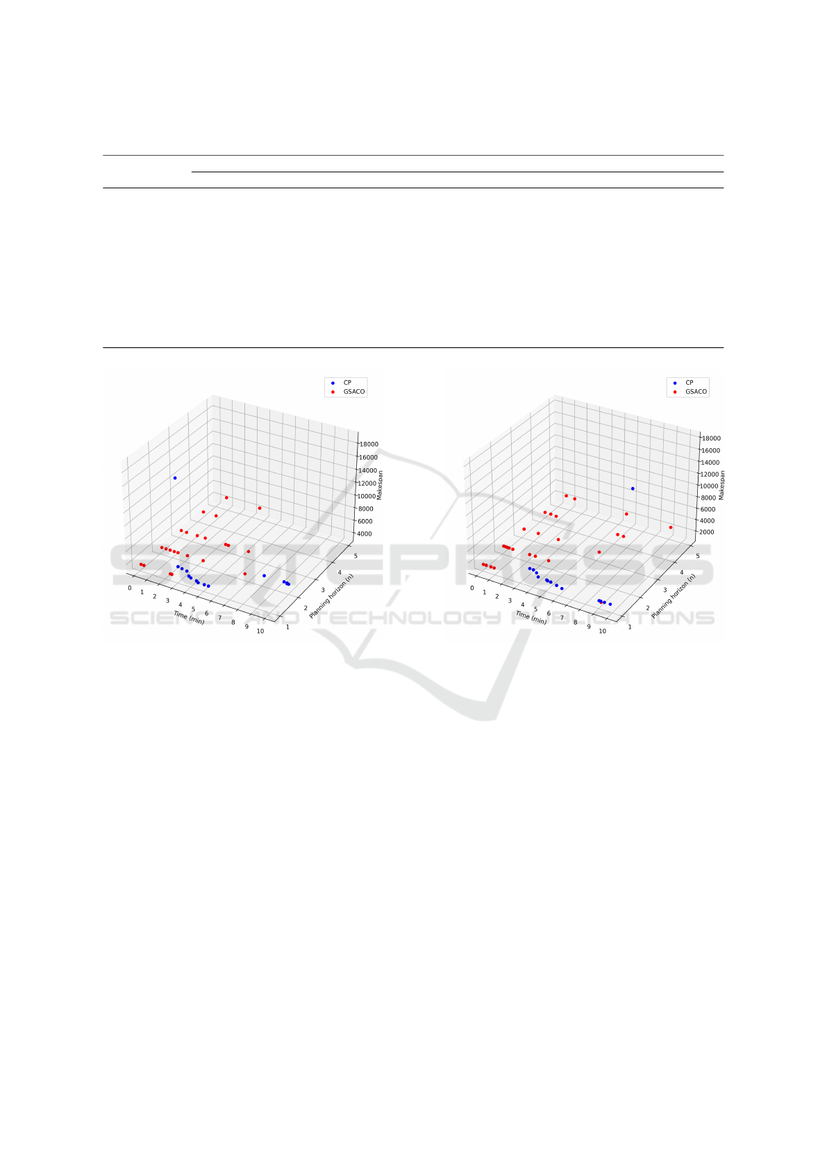
Table 7: SMSP results obtained with CP and GSACO.

1 min 3 min 5 min 7 min 9 min

n Scenario CP GSACO CP GSACO CP GSACO CP GSACO CP GSACO

LV/HM - 3735 18572 3725 3746 3725 3723 3725 3723 3725

HV/LM - 1405 - 1405 2242 1405 1609 1405 1600 1405

LV/HM - 3773 - 3751 - 3750 - 3739 4398 3739

HV/LM - 1653 - 1644 - 1611 - 1611 - 1611

LV/HM - 3880 - 3867 - 3836 - 3834 - 3834

HV/LM - 1902 - 1889 - 1889 - 1876 - 1876

LV/HM - 4578 - 4540 - 4540 - 4540 - 4540

HV/LM - 2207 - 2113 - 2113 - 2093 - 2093

LV/HM - 4680 - 4680 - 4553 - 4553 - 4553

HV/LM - 2667 - 2566 - 2566 - 2518 - 2518

(a) LV/HM scenario (b) HV/LM scenario

Figure 7: Makespan improvements of schedules for SMSP instances obtained with CP and GSACO.

ﬁnds outliers as its ﬁrst solutions. This phenomenon

occurs for the planning horizons n = 1 and n = 2 on

the LV/HM or HV/LM scenario, respectively, where

the latter schedule of makespan 17664 is found after

more than 9 minutes and thus not listed in Table 7.

6 CONCLUSION

Modern semiconductor fabs are highly complex and

dynamic production environments, whose efﬁcient

operation by means of automated scheduling and con-

trol systems constitutes a pressing research challenge.

In this work, we model the production processes of

large-scale semiconductor fabs in terms of the well-

known FJSSP. In contrast to classical FJSSP bench-

marks, this leads to large-scale scheduling problems,

even if short planning horizons cover only a fraction

of the long production routes with hundreds of opera-

tions. The resulting size and complexity of large-scale

SMSP instances exceed the capabilities of common

FJSSP solving methods. We thus propose the GSACO

algorithm combining probabilistic operation sequenc-

ing with greedy machine assignment. Its efﬁcient

implementation utilizing tensor operations and par-

allel ant simulations enables GSACO’s convergence

to high-quality solutions in short time. In this way,

GSACO overcomes the scalability limits of exact op-

timization by means of a state-of-the-art CP approach

and achieves the performance required for frequent

re-scheduling in reaction to process deviations.

While simpliﬁed FJSSP models of semiconduc-

tor manufacturing processes provide insights regard-

ing the scalability of scheduling methods, in future

work, we aim at extending GSACO to incorporate

the speciﬁc conditions and functionalities of tools per-

forming the production operations. Such features in-

clude, e.g., machine setups to be equipped before

A Greedy Search Based Ant Colony Optimization Algorithm for Large-Scale Semiconductor Production

147

performing operations, preventive maintenance pro-

cedures for which a machine needs to stay idle, and

batch processing capacities to handle several produc-

tion lots in one pass. In practice, these speciﬁcs matter

for machine assignment strategies and should also be

reﬂected in the respective greedy phase of GSACO.

Our second target of future work concerns the uti-

lization of schedules found by GSACO for decision

making and control within simulation models of semi-

conductor fabs. This goes along with the extension of

optimization objectives to practically relevant perfor-

mance indicators, such as deadlines for the comple-

tion of jobs and minimizing the tardiness. In view of

the dynamic nature of real-world production opera-

tions and unpredictable stochastic events, quantifying

the improvements by optimized scheduling methods

requires their integration and evaluation in simulation.

ACKNOWLEDGEMENTS

This work has been funded by the FFG project

894072 (SwarmIn). We are grateful to the anonymous

reviewers for constructive comments that helped to

improve the presentation of this paper.

REFERENCES

Abdel-Basset, M., Ding, W., and El-Shahat, D. (2021).

A hybrid Harris Hawks optimization algorithm with

simulated annealing for feature selection. Artiﬁcial

Intelligence Review, 54(1):593–637.

Arnaout, J.-P., Musa, R., and Rabadi, G. (2014). A two-

stage ant colony optimization algorithm to minimize

the makespan on unrelated parallel machines—part II:

enhancements and experimentations. Journal of Intel-

ligent Manufacturing, 25(1):43–53.

Behnke, D. and Geiger, M. J. (2012). Test instances for

the ﬂexible job shop scheduling problem with work

centers. Technical Report RR-12-01-01, Helmut-

Schmidt-Universit

at.

Brandimarte, P. (1993). Routing and scheduling in a ﬂex-

ible job shop by tabu search. Annals of Operations

Research, 41(3):157–183.

Dorigo, M. and St

utzle, T. (2019). Ant colony optimiza-

tion: overview and recent advances. In Handbook of

Metaheuristics, pages 311–351. Springer.

El Khoukhi, F., Boukachour, J., and El Hilali Alaoui, A.

(2017). The “dual-ants colony”: a novel hybrid ap-

proach for the ﬂexible job shop scheduling problem

with preventive maintenance. Computers & Industrial

Engineering, 106:236–255.

Fattahi, P., Saidi Mehrabad, M., and Jolai, F. (2007). Mathe-

matical modeling and heuristic approaches to ﬂexible

job shop scheduling problems. Journal of Intelligent

Manufacturing, 18(3):331–342.

Fontes, D. B., Homayouni, S. M., and Gonc¸alves, J. F.

(2023). A hybrid particle swarm optimization

and simulated annealing algorithm for the job shop

scheduling problem with transport resources. Euro-

pean Journal of Operational Research, 306(3):1140–

1157.

Gao, L., Peng, C. Y., Zhou, C., and Li, P. G. (2006). Solv-

ing ﬂexible job shop scheduling problem using gen-

eral particle swarm optimization. In Proceedings of

the 36th Conference on Computers & Industrial Engi-

neering, pages 3018–3027.

Gedik, R., Kalathia, D., Egilmez, G., and Kirac, E. (2018).

A constraint programming approach for solving unre-

lated parallel machine scheduling problem. Comput-

ers & Industrial Engineering, 121:139–149.

Ho, N. B., Tay, J. C., and Lai, E. M.-K. (2007). An ef-

fective architecture for learning and evolving ﬂexible

job-shop schedules. European Journal of Operational

Research, 179(2):316–333.

Khelifa, B. and Laouar, M. R. (2020). A holonic intelligent

decision support system for urban project planning by

ant colony optimization algorithm. Applied Soft Com-

puting, 96:106621.

Kopp, D., Hassoun, M., Kalir, A., and M

onch, L. (2020).

SMT2020—a semiconductor manufacturing testbed.

IEEE Transactions on Semiconductor Manufacturing,

33(4):522–531.

Kov

acs, B., Tassel, P., and Gebser, M. (2023). Optimiz-

ing dispatching strategies for semiconductor manufac-

turing facilities with genetic programming. In Pro-

ceedings of the Genetic and Evolutionary Computa-

tion Conference, pages 1374–1382. ACM.

Ku, W. and Beck, C. (2016). Mixed integer programming

models for job shop scheduling: a computational anal-

ysis. Computers & Operations Research, 73:165–173.

Leung, C. W., Wong, T., Mak, K.-L., and Fung, R. Y.

(2010). Integrated process planning and scheduling

by an agent-based ant colony optimization. Comput-

ers & Industrial Engineering, 59(1):166–180.

Li, J.-Q., Pan, Q.-K., and Tasgetiren, M. F. (2014). A

discrete artiﬁcial bee colony algorithm for the multi-

objective ﬂexible job-shop scheduling problem with

maintenance activities. Applied Mathematical Mod-

elling, 38(3):1111–1132.

Li, L., Keqi, W., and Chunnan, Z. (2010). An improved

ant colony algorithm combined with particle swarm

optimization algorithm for multi-objective ﬂexible job

shop scheduling problem. In Proceedings of the Inter-

national Conference on Machine Vision and Human-

machine Interface, pages 88–91. IEEE.

Li, Q., Ning, H., Gong, J., Li, X., and Dai, B. (2021).

A hybrid greedy sine cosine algorithm with differen-

tial evolution for global optimization and cylindric-

ity error evaluation. Applied Artiﬁcial Intelligence,

35(2):171–191.

Luo, D., Wu, S., Li, M., and Yang, Z. (2008). Ant colony

optimization with local search applied to the ﬂexi-

ble job shop scheduling problems. In Proceedings

of the International Conference on Communications,

Circuits and Systems, pages 1015–1020. IEEE.

SIMULTECH 2024 - 14th International Conference on Simulation and Modeling Methodologies, Technologies and Applications

148

Meng, L., Zhang, C., Ren, Y., Zhang, B., and Lv, C. (2020).

Mixed-integer linear programming and constraint pro-

gramming formulations for solving distributed ﬂexi-

ble job shop scheduling problem. Computers & In-

dustrial Engineering, 142:106347.

Mohd Tumari, M. Z., Ahmad, M. A., Suid, M. H., and

Hao, M. R. (2023). An improved marine preda-

tors algorithm-tuned fractional-order PID controller

for automatic voltage regulator system. Fractal and

Fractional, 7(7):561.

Papadimitriou, C. H. and Steiglitz, K. (1982). Combi-

natorial Optimization: Algorithms and Complexity.

Prentice-Hall.

Perron, L., Didier, F., and Gay, S. (2023). The CP-SAT-

LP solver (invited talk). In Proceedings of the 29th

International Conference on Principles and Practice

of Constraint Programming, pages 3:1–3:2. Leibniz

International Proceedings in Informatics.

Rizzoli, A. E., Montemanni, R., Lucibello, E., and Gam-

bardella, L. M. (2007). Ant colony optimization for

real-world vehicle routing problems: from theory to

applications. Swarm Intelligence, 1:135–151.

Rugwiro, U., Gu, C., and Ding, W. (2019). Task schedul-

ing and resource allocation based on ant-colony opti-

mization and deep reinforcement learning. Journal of

Internet Technology, 20(5):1463–1475.

Saidi-Mehrabad, M. and Fattahi, P. (2007). Flexible job

shop scheduling with tabu search algorithms. Interna-

tional Journal of Advanced Manufacturing Technol-

ogy, 32:563–570.

Shang, X. (2023). A study of deep learning neural net-

work algorithms and genetic algorithms for FJSP.

Journal of Applied Mathematics, 2023:4573352:1–

4573352:13.

Sobeyko, O. and M

onch, L. (2016). Heuristic approaches

for scheduling jobs in large-scale ﬂexible job shops.

Computers & Operations Research, 68:97–109.

ockermann, P., Immordino, A., Altenm

uller, T., Seidel,

G., Gebser, M., Tassel, P., Chan, C. W., and Zhang,

F. (2023). Dispatching in real frontend fabs with in-

dustrial grade discrete-event simulations by deep rein-

forcement learning with evolution strategies. In Win-

ter Simulation Conference, pages 3047–3058. IEEE.

utzle, T. and Dorigo, M. (1999). ACO algorithms for the

traveling salesman problem. In Evolutionary Algo-

rithms in Engineering and Computer Science, pages

163–183. John Wiley & Sons.

Suid, M. H. and Ahmad, M. A. (2023). A novel hybrid of

nonlinear sine cosine algorithm and safe experimenta-

tion dynamics for model order reduction. Journal for

Control, Measurement, Electronics, Computing and

Communications, 64(1):34–50.

Tassel, P., Kov

acs, B., Gebser, M., Schekotihin, K.,

ockermann, P., and Seidel, G. (2023). Semicon-

ductor fab scheduling with self-supervised and rein-

forcement learning. In Winter Simulation Conference,

pages 1924–1935. IEEE.

Thammano, A. and Phu-ang, A. (2013). A hybrid artiﬁ-

cial bee colony algorithm with local search for ﬂexi-

ble job-shop scheduling problem. Procedia Computer

Science, 20:96–101.

urkyılmaz, A., S¸envar,

O.,

Unal,

I., and Bulkan, S. (2020).

A research survey: heuristic approaches for solving

multi objective ﬂexible job shop problems. Journal of

Intelligent Manufacturing, 31(8):1949–1983.

Wang, J., Osagie, E., Thulasiraman, P., and Thulasiram,

R. K. (2009). HOPNET: a hybrid ant colony optimiza-

tion routing algorithm for mobile ad hoc network. Ad

Hoc Networks, 7(4):690–705.

Wang, L., Cai, J., Li, M., and Liu, Z. (2017). Flexi-

ble job shop scheduling problem using an improved

ant colony optimization. Scientiﬁc Programming,

2017:9016303:1–9016303:11.

Xie, J., Gao, L., Peng, K., Li, X., and Li, H. (2019). Review

on ﬂexible job shop scheduling. IET Collaborative

Intelligent Manufacturing, 1(3):67–77.

Xing, L.-N., Chen, Y.-W., Wang, P., Zhao, Q.-S., and

Xiong, J. (2010). A knowledge-based ant colony op-

timization for ﬂexible job shop scheduling problems.

Applied Soft Computing, 10(3):888–896.

Xiong, H., Shi, S., Ren, D., and Hu, J. (2022). A survey of

job shop scheduling problem: the types and models.

Computers & Operations Research, 142:105731.

A Greedy Search Based Ant Colony Optimization Algorithm for Large-Scale Semiconductor Production

149