Intelligent Sampling System for Connected Vehicle Big Data

Omar Makke

1 a

, Syam Chand

2 b

, Vamsee Krishna Batchu

2 c

, Oleg Gusikhin

1 d

and Vicky Svidenko

1 e

Ford Motor Company, U.S.A.

Ford Motor Company, India

Keywords:

Connected Vehicles, Sampling, Big Data, Large Language Model Application, Generative AI.

Abstract:

The impact of connected vehicle big data on the automotive industry is signiﬁcant. Big data offers data scien-

tists the opportunity to explore and analyze vehicle features and their usage thoroughly to assist in optimizing

existing designs or offer new features. However, the downside of big data is its associated cost. While storage

tends to be cheap, data transmission and computational resources are not. Speciﬁcally, for connected vehicle

data, even when unstructured data is excluded, the data size can still increase by several terabytes a day if

one is not careful about what data to collect. Therefore, it is advisable to apply methods which help avoiding

collecting redundant data to reduce the computation cost. Furthermore, some data scientists may be tempted

to calculate “exact” metrics when the data is available, partly because applying statistical methods can be

tedious, which can exhaust the computational resources. In this paper we argue that intelligent sampling sys-

tems which centralize the sampling methods and domain knowledge are required for connected vehicle big

data. We also present our system which assists interested parties in performing analytics and provide two case

studies to demonstrate the beneﬁts of the system.

1 INTRODUCTION

As connected vehicles become more mainstream, the

demand for acquiring and accessing connected vehi-

cle data has been increasing. Even though a vehi-

cle equipped with few cameras has the potential to

generate terabytes of data each day, as of today, only

few megabytes of structured data are sent over the air

to the cloud due to the relatively large cost of data

transmission. Larger volumes of data are usually sent

over WIFI if the vehicle is conﬁgured to connect to

the owner’s network, which is usually not the case.

Nevertheless, with millions of vehicles present on the

road, and due to the increment of connected vehicle

features, the data size will grow at a minimum of

polynomial rate, as will be shown later. With this data

growth, reliance on sampling techniques will become

important to efﬁciently build models. More discus-

sion on the role of sampling in big data can be found

in (Albattah, 2016).

https://orcid.org/0000-0002-7295-751X

https://orcid.org/0009-0003-0195-3807

https://orcid.org/0009-0008-9825-8339

https://orcid.org/0000-0001-6943-4227

https://orcid.org/0009-0009-9458-1507

In general, obtaining data from a vehicle has the

following challenges. Transmission cost, bandwidth

limitations, storage, computational costs, and admin-

istrative costs such as adhering to regulations, man-

aging access, etc. Using today’s technologies, engi-

neers can put data request orders to specify the signals

that must be collected (Rocci et al., 2021). In many

cases, different requests can specify common signals

and thus creating data duplication in the cloud. Fur-

thermore, the data request owners may not be aware

of additional related signals which may be of inter-

est. Vehicle signal speciﬁcation standard (COVESA,

2024) attempts to mitigate this problem and provide

a common language for signals. While this covers

the “common” signals used, each Original Equipment

Manufacturer (OEM) has plethora of other architec-

ture speciﬁc signals. Different vehicle types can have

different vehicle architectures, and for the same vehi-

cle type, its architecture can vary among model years.

Therefore, identifying which signals are needed for

a representative study is not trivial since the signals

can vary between model years and can vary between

vehicles having the same model year.

Another challenge arises in determining how

much data to collect and from how many vehicles.

150

Makke, O., Chand, S., Batchu, V., Gusikhin, O. and Svidenko, V.

Intelligent Sampling System for Connected Vehicle Big Data.

DOI: 10.5220/0012813500003756

Paper published under CC license (CC BY-NC-ND 4.0)

In Proceedings of the 13th International Conference on Data Science, Technology and Applications (DATA 2024), pages 150-158

ISBN: 978-989-758-707-8; ISSN: 2184-285X

Engineers and data scientists are tempted to collect

“as much data as possible” which can be costly, or for

simplicity, they may sample from arbitrarily selected

vehicles. They usually do not have all the knowledge

about the general demographics, geographical simi-

larities, vehicle conﬁgurations, etc. as these change

over time. Therefore, it is important to have a cen-

tralized system which assists in collecting the proper

amount data from the required signals sampled cor-

rectly. Otherwise, studies or machine learning mod-

els can be biased and under-perform, as can be shown

in (Hasanin et al., 2019) and (Johnson and Khoshgof-

taar, 2020).

To solve this problem, we developed an intelli-

gent sampling system for connected vehicle feature

analytics which combines connected vehicles domain

knowledge and analytical results with data sampling

techniques, while balancing the budget with the de-

sired statistical signiﬁcance whenever possible. It as-

sists the users in determining which signals to use,

sampling technique, and in choosing a sample suit-

able for their studies while meeting their budget con-

straints.

This paper is organized as follows. Section 2 de-

scribes common technologies used in vehicles, and

motivates the need for an intelligent sampling sys-

tem. Section 3 describes our system architecture and

components. Section 4 demonstrates using the sys-

tem for analyzing feature usage on different types of

roads. Section 5 describes a case which models fuel

consumption as a function of tire pressure. Section 6

concludes the paper.

2 BACKGROUND

Big data challenges related to our work have been

known for several years, even before cloud solutions

became powerful. As computational power improved,

data collection also increased, and therefore, these

challenges remain. An obvious approach to deal with

the computational burden created by big data is sam-

pling. What is not obvious is how to perform the

sampling. For example, in (Casamayor-Pujol et al.,

2023), the authors designed a scalable “Intelligent

Sampling” method to assist in scheduling workloads

in large scale heterogeneous computing continuum.

This, of course, is abstracted from the end users who

are interested in building models, which serves as a

suitable example of an intelligent sampling system.

A comprehensive list of sampling techniques is found

in (Djouzi et al., 2023). Some of these methods are

very well known. We review some of the fairly re-

cent methods in adaptive sampling. In (John and

Langley, 1996), the authors introduced a progressive

sampling method and the concept of “Probably Close

Enough” (PCE). The idea behind PCE is to obtain a

good enough sample such that it is very unlikely to

improve a mining algorithm any further by using the

entire dataset. The authors discussed static versus dy-

namic sampling and their work aims to deal with big

data efﬁciently. In (Satyanarayana, 2014), the authors

proposed Generalized Dynamic Adaptive Sampling

(GDAS), an adaptive sampling technique to tackle

the limitations in progressive sampling, listed in their

work. In (Djouzi et al., 2022), the authors proposed

a new adaptive sampling method, Subsampled Dou-

ble Bootstrap GDAS (SDBGDAS) method, which is

an improvement over GDAS (Satyanarayana, 2014)

method, which allows the scaling of adaptive methods

to big data. In (Loyola R et al., 2016), various sam-

pling methods are discussed and the authors propose

a Smart Sampling and Incremental Function Learning

Algorithm to ﬁnd a Probably Approximately Correct

Computation (PACC) regression model.

Other work, such as in (Zhang and Wang, 2021),

(Ai et al., 2021), investigated methods to deal with

distributed and massive data. The idea is to opti-

mally select a distributed sub-data, for which sum-

mary statistics are calculated on the edge and sent to

a central server or to build generalized linear models

(GLM). Fuzzy methods are also proposed to reduce

sample size such as in (He et al., 2015).

Whether simple random sampling techniques are

used, or advanced methods, it is clear that challenges

arise when dealing with big data, and good sampling

techniques help address these challenges. As noted

earlier, the data size of connected vehicle data in

the cloud grows at least polynomially (ignoring any

changes in regulations, consent agreements, etc.). A

proof is offered here before proceeding to the next

section.

2.1 Polynomial Growth of Connected

Vehicle Data

To motivate the need for intelligent sampling systems,

we ﬁrst show that the data will grow at polynomial

rate during the next few years. Let S

be the number

of connected vehicles sold in year y, and assume that

< y

=⇒ |S

| < |S

|. In other words, the sales of

connected vehicles each year are more than the pre-

vious year (unsaturated market). Note that we only

consider connected vehicles. Therefore, the assump-

tion |S

| <= |S

| holds until almost all vehicles on

the road are connected vehicles. Let d

be the amount

of data collected from model year y

. Assuming d

is proportional to S

, we have y

< y

=⇒ d

< d

Intelligent Sampling System for Connected Vehicle Big Data

151

meaning, each new year we collect more data than

the previous year. Under these assumptions, we now

prove that the data size grows at least polynomially

with the years.

Let I be an enumeration set of all years under

which the assumptions hold. Let ∆

= d

− d

i−1

, the

increment of collected data for year y

, i ∈ I. For all

the years, while the market is not saturated with con-

nected vehicles, there exists a year for which the in-

crement in data collection ∆

min

is minimal.

Then

∑

i∈I

= d

+ d

+ ... (1)

∑

i∈I

= d

+ d

+ ∆

+ d

+ ∆

+ d

+ ∆

+ ... (2)

(3)

But

i+1

> d

+ ∆

min

> d

i−1

+ 2∆

min

(4)

Therefore

∑

i∈I

≥ d

+ d

+ ∆

min

+ d

+ 2∆

min

+ d

+ 3∆

min

...

(5)

∑

i∈I

≥ |I|d

∑

i∈I

i∆

min

(6)

Letting N = |I|, the number of included years, then the

partial increment of data ∆(N) at year N from year y

∆(n) =

∑

n=1

n∆

min

(7)

∆(n) = ∆

min

N(N + 1)

(8)

Hence, the data size grows with the years, following

at least a polynomial of order 2. □

Therefore, it is important to build a system which

efﬁciently selects a representative samples to han-

dle the large amount of actual and expected data.

For example, the systems described in (Makke and

Gusikhin, 2018) and (Tran et al., 2024) will require

less data to build the desired models and to update

them on a regular basis, which makes the cost of

“live” services feasible.

3 SYSTEM DESCRIPTION

To address the issues listed above we propose a sys-

tem which assists in performing “Connected Vehicle

Feature Analytics” deﬁned below, by combining sam-

pling techniques with domain knowledge retrieval,

while simultaneously considering any known system

or budget constraint.

Deﬁnition 3.1. Connected Vehicle Feature Analytics

(CVFA) refers to the analysis of the performance and

usage of the vehicle features within the vehicle pop-

ulation. The objective is to generate actionable in-

sights for engineering, marketing and product devel-

opment, leveraging connected vehicle technology, do-

main knowledge, and data science.

Signals Lab Reports

Spec

Signal

Recommender

(LLM)

Cost Es�mator

Constraints

Historical Orders

Wish List

Minimum Signals

Required

Jus�ﬁca�on For Data Collec�on

(Natural Language)

List of model speciﬁc signal names to sample

Budget

Figure 1: Architecture of Signal Recommender.

In comparison to “connected services”, features such

as remote start from mobile phone and prognostics,

which are tailored to individual vehicles, are not

CVFA since CVFA focuses on the broader trends.

The proposed system is divided into two main

components. The ﬁrst is the Signal Recommender

component which focuses on assisting the users with

choosing the correct signals for their studies while

adhering to any system or business constraints. The

second is the Intelligent Data Collection component

which, once signals are known, assists the users in

sampling the data sources using one of the many sam-

pling techniques. These components are discussed in

details below.

3.1 Signal Recommender

The architecture for the Signal Recommender is

shown in Figure 1. The user starts by describing the

use case using natural language. This step is required

before the data collection is approved to ensure that

privacy rules and regulations are met, and that the pro-

posed use case ﬁts within the driver’s consent agree-

ment. The user of the system also selects the sig-

nals of interest by their “standard” name such as VSS

(COVESA, 2024). This is important because the ac-

tual signal names can change based on the vehicle ar-

chitecture. For example, an 8 bits temperature signal

on CAN bus may have a sufﬁx of “ 8”, but on vehicles

with Automotive Ethernet (IEEE Standards Associa-

DATA 2024 - 13th International Conference on Data Science, Technology and Applications

152

tion, 2015), it may be 16 bits. The user may not know

which model year this change took effect. The user

also speciﬁes a budget which can be approximated as

dollars per megabytes of data.

This information, along with vehicle speciﬁcation

documents, network signal speciﬁcations, relevant lab

reports, and historical data collection orders are fed

into a signal recommender. This can be either a classi-

cal recommender based on knowledge databases such

as vehicle ontology, or it can be implemented with the

assistance of a Large Language Model (LLM) (Ope-

nAI, 2023), (Google, 2023). We ﬁnd that an LLM

can easily recommend possible relevant signals when

such information is provided. The LLM has the ad-

vantage of being able to read the use case justiﬁ-

cation to understand the issue and match that with

other documents using Retrieval Augmented Gener-

ation (RAG) techniques to identify other possible sig-

nals.

The cost estimator looks up the type of signal

and its speciﬁcation and provides a cost estimate for

adding that signal to the study. For example, a Door

Switch signal is an event driven signal where as a

transmission output speed is an analog signal that can

be collected at around 10Hz. Ambient temperature is

available at 1Hz but the signal does not have to be col-

lected at that rate unless a speciﬁc study related to the

performance of the sensor is required.

The constraints block imposes any constraints on

the system, such as no more than 10 Mb can be trans-

ferred from vehicles with 3G connection, and no more

than 50 Mb can be transferred from vehicles with 4G

connections. This is important because at any point

in time, there are vehicles of different ages and tech-

nologies on the road. Usually, it sufﬁces to choose a

speciﬁc model year for the study, but in some cases

a study can span different model years such as when

investigating tire pressure, general vehicle usage, etc.

The output of this component is a list of signals

to sample along with the desired sample rate, and this

list is an input to the next component.

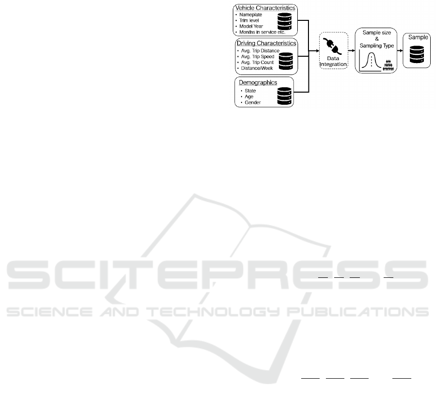
3.2 Signal Sampling and Collection

The Signal Sampling and Collection component com-

prehensively analyze driving characteristics, vehicle

attributes, and demographic data to determine the ap-

propriate sampling size and type, as shown in Figure

2. More dimensions are available and additional ones

can be added over time, such as the study shown in

Section 4. The selection of these set of factors is en-

tirely dependent on the objective of data collection.

By integrating these key factors, the system aims to

generate a sample that is not only statistically signiﬁ-

cant in size but also representative of the wider popu-

lation.

Figure 2: Architecture of Signal Sampling and Collection.

3.3 Sample Size

In the case of connected vehicles it’s nearly impos-

sible to collect data from all the vehicles and hence

the population size is unknown. There are difference

approaches to estimate the sample size based on the

distribution of selected continuous and discrete sam-

pling parameters. For continuous sampling parame-

ters like average trip distance and given the popula-

tion is unknown, the sample size is estimated (Nan-

jundeswaraswamy and Divakara, 2021) by,

= Z

max



........



Z: Z – statistic value for the required conﬁdence level

: Variability of the sampling parameter

e: Maximum allowable error

For discrete sampling parameters like model year

of vehicle and given the population is unknown, the

sample size is estimated (Louangrath, 2019) by,

= Z

max



........



Z: Z – statistic value for the required conﬁdence level

p: Proportion of the class in the sampling variable

q = (1-p)

e: Maximum allowable error.

The overall sample size for the study with a com-

bination of continuous and discrete sampling parame-

ters has been chosen as the maximum of the estimated

individual sample sizes.

= max(n

, n

)

: minimum sample size required to account for the

variability in continuous sampling attributes.

: minimum sample size required to account for the

variability in discrete sampling attributes

Thus, the maximum allowable error and conﬁ-

dence level can be traded off with the available budget

before data is collected.

Intelligent Sampling System for Connected Vehicle Big Data

153

3.4 Sampling Type

Figure 3: Stratiﬁed Random Sampling.

Selecting a sample that represents the population is

as important as collecting data from statistically sig-

niﬁcant sample size. Once the sample size is esti-

mated, it is important to identify a set of vehicles that

represent the distribution of the targeted population,

and the sampling methodology depending on objec-

tive of the study (Elﬁl and Negida, 2016). We ﬁnd

that ’Stratiﬁed Random Sampling’ method is effec-

tive as it balances the complexity of sampling with

the intended use of data, since in most cases all sub-

jects in the targeted population have equal chances to

be selected. Otherwise, we choose non-probabilistic

sampling - “Judgmental Sampling”.

Stratiﬁed sampling is a probabilistic sampling

method which is based on dividing a population into

strata of homogeneous members, and members of the

sample are selected randomly from these strata. For

example, if we want to collect data to study usage of

washer ﬂuid, it is important to select driving charac-

teristics that have high correlation with washer ﬂuid

usage like average trip speed, average trip duration

and state in which vehicle is being driven. The en-

tire population is divided into homogeneous strata and

samples would be picked from each strata propor-

tionately as shown in Figure 3. Population(N)=1500,

Sample Size (n) = 300, and Strata Multiplier = 0.2

(

This methodology would ensure that data is repre-

senting the population and sample size is statistically

signiﬁcant.

As more strata are discovered, their descriptions

and sample sizes are added to our system, exposed

to the LLM, thus allowing future users to select from

these strata, and thus allowing the system capability

to naturally grow with time.

3.5 Logical Grouping of Events

In addition to sampling data from the vehicles, the

system is setup to sample from existing connected ve-

hicle data. Millions of vehicles on the road sending

at least a Megabyte of data a week raises challenges

in managing the collected data. Even if querying the

entire data set is possible, that can be very expen-

sive. Therefore, it is important to store the data in a

form that can be sampled correctly based on different

needs. Logically, the data is partitioned using event

Ids as shown in Figure 4. When the controller send-

ing the data boots up, it generates a unique identiﬁca-

tion number by hashing its VIN and a randomly gen-

erated number. Figure 4 shows an example of these

events, some of which are disjointed such as “Drive

Mode” and “Park mode”, and some of which are hi-

erarchical such as “Ignition Id” and “Drive Cycle Id”.

Then, as an example, suppose there is also an “Abs

Id”, an event indicating an anti-lock braking system

actuation event. The sampling can be limited to grab

data from all data which have “Ignition Id” that has at

least 1 “Abs Id” event. Furthermore, the sampling can

be performed so that (1) Either data is sampled ran-

domly from the set of all data which has in its “Igni-

tion Id” event at least one “Abs Id” event, (2) or sam-

ple a small subset of “Ignition Id” events which have

at least one “Abs Id” event, and then for each sam-

ple “Ignition Id”, grab all its data. This is important

if the data leading to an event is important, and must

be complete. Note that the LLM plays an important

role here if the users of the system do not know the

details on when the signal is available. For example,

it may be trivial that cruise control is only available

when “Drive Cycle Id” is present, but the user of the

system may not know that there is a “Drive Cycle Id”

for use, especially when there are many other event

identiﬁcation numbers present. The speciﬁcation of

the tagging system are fed into the LLM which then

recommends to the users to limit the sampling to the

events tagged with “Drive Cycle Id”. In addition to

the case studies that will be discussed in this paper,

other examples which use this system can be found in

(Beyel et al., 2024) and (Beyel. et al., 2023).

4 CASE STUDY 1: GEO-SPECIAL

FEATURE USAGE

Consider the following scenario. An OEM needs to

conduct a study on how a speciﬁc feature is used on

different roads. In order to do that, the OEM must an-

alyze how many kilometers a vehicle spends on dif-

ferent types of roads. Here, the type of roads are

as deﬁned by Open Street Map (OSM) (Open Street

Map, 2024). Suppose also that the data is already

collected at a rate of 1 sample every 30 seconds (a

constraint) as described in the previous section. To

determine how man kilometers on average vehicles

drive on each type of road, GPS coordinates, vehicle

speed and vehicle type are needed. Then, for every

30 seconds, and a speed sample v

we estimate total

kilometers driven to be

DATA 2024 - 13th International Conference on Data Science, Technology and Applications

154

Igni�on

Controller

Wakes up

Drive Mode

Begins

Drive

Mode

Ends

Igni�on

Oﬀ

Drive Mode

Begins

Drive

Mode

Ends

Controller

Sleeps

Boot ID

Igni�on ID

Drive Cycle ID

Park ID

Stop ID

Drive Cycle ID

Messages

contain

Boot id

Messages

contain:

Boot ID

Igni�on ID

Messages

contain:

Boot ID

Igni�on ID

Drive Mode ID

Messages

contain:

Boot ID

Igni�on ID

Park Cycle ID

Messages

contain:

Boot ID

Igni�on ID

Stop Cycle ID

Messages

contain:

Boot ID

Stop Cycle ID

Messages

contain:

Boot ID

Igni�on ID

Drive Cycle ID

Figure 4: Data is tagged with various event identiﬁcation numbers to make sampling more efﬁcient.

total

∑

× 0.0083h (9)

Equation (9) works as long as all the samples i ∈ I

are chosen, where I is the set of all measurements

of vehicle speed. However, millions of data points

can exist at every 30 seconds interval, and perform-

ing Geo-special queries to map each GPS recording

to the nearest road type is computationally expensive.

Therefore, sampling is required.

Remark: Note that the experiments conducted can be

repeated for each Strata (vehicle type). The results

shown here, however, are for the entire dataset for

conﬁdentiality reasons.

To demonstrate the effectiveness of sampling con-

necting vehicle data, two experiments are performed.

In the ﬁrst experiment, 0.01% of the data over a year

(3 Million points), and in the other, around 0.00005%

of the data over year (around 10k data points). Boot-

strap method is used, and each experiment is repeated

32 times, and the mean and standard deviation are av-

eraged over the 32 trials.

Table 1 shows the distribution of kilometers driven

per Open Street Map road type. The road type is cho-

sen to be the closest match on OSM within 100 me-

ters to the logged GPS coordinates. Table 2 shows

that when 3 million samples where used, the stan-

dard deviation was every small. When the sample size

is reduced to 10k, the standard deviation increased.

However, as shown in Table 3, the percentage change

between using 3 million samples and 10k samples is

negligible. It is worth noting that the query duration

dropped from around 2 hours to around 5 minutes.

In this case study, the signals were trivial to iden-

tify, and the study was straight forward. The compo-

nent shown in Figure 2 is still used, except the sam-

pling is performed on already existing data.

Remark: Running the query on the entire data set

Table 1: Mean % of the trials measuring kilometers driven

on different road types using different sample sizes.

Road Type % (3M Samples) % (10k Samples)

Motorway 23.92 24.1

MW Junction 3.97 3.88

MW Link 10.75 11.1

Trunk 5.3 5.05

Trunk Link 0.92 0.85

Primary 9.71 9.83

Secondary 10.34 10.18

Tertiary 9.69 9.9

Others 25.38 25.11

would time out after 2 hours, and it was not possi-

ble to obtain the metrics from the entire data set. The

larger set (3 million samples) was heuristically setup

so that the query ﬁnishes in approximately 2 hours

before the query terminates.

5 CASE STUDY 2: IMPACT OF

TIRE PRESSURE ON FUEL

ECONOMY

In this study, we are interested to ﬁnd the relation

between tire pressure and fuel economy. Using the

LLM, we ﬁnd that tire pressure signals and fuel econ-

omy signals are common across wide range of vehi-

cle older vehicle and all recent vehicles. Furthermore,

from the CAN Database, the LLM identiﬁed that not

all the signals have the same unit (depending on the

architecture and the country). The data size is in the

order of tens of terabytes. Although this is not a prob-

lem at all for Big-Query, an organization may throttle

the consumption of computational resources per user

Intelligent Sampling System for Connected Vehicle Big Data

155

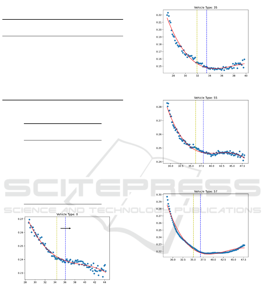
Table 2: Standard deviation of the trials shown in Table 1.

Smaller data sets are still accurate.

Road Type (3M Samples) (10k Samples)

Motorway 0.02 2.37

MW Junction 0.01 0.29

MW Link 0.01 0.48

Trunk 0.01 0.37

Trunk Link 0.01 0.09

Primary 0.01 0.64

Secondary 0.01 0.51

Tertiary 0.01 0.49

Others 0.02 1.1

Table 3: Difference between the results using different sam-

ple sizes.

Road Type % Difference

Motorway -0.01

MW Junction 0.02

MW Link -0.03

Trunk 0.05

Trunk Link 0.08

Primary -0.01

Secondary 0.02

Tertiary -0.02

Others 0.01

% Gas Tank

PSI

Normal Region

Saving

Opportunity

Ignored Region

Figure 5: Example of fuel consumption as a function of tire

pressure for an arbitrary vehicle type.

to prevent cost runaway. Therefore, sampling the data

is desired. For each of the vehicle types identiﬁed un-

der “Vehicle Characteristics” in Figure 2, 5% of the

data is sampled. The maximum reported ”Fuel Level”

for each vehicle type is considered to be a full tank at

100%, and then all fuel level measurements are nor-

malized by that maximum for each vehicle type. For

each trip with “Ignition Id” present, the ﬁrst and last

tire pressure measurements from all 4 tires are taken

and averaged (average of 8 measurements). The av-

% Gas Tank

(a) Heavy Vehicle.

% Gas Tank

(b) Medium Vehicle.

% Gas Tank

Figure 6: Graphs showing the performance of 3 classes of

vehicles. The area on the left of the dashed line is common.

The area on the right side of the lines is ignored.

erage tire pressure is assumed to be the tire pressure

for the trip, converted to PSI. The x-axis in Figure 5

represents the average tire pressure for each trip. The

x-axis is quantized by steps of 0.2 PSI, so that each

two consecutive integer PSI measurements on the x-

axis constitute 5 bins.

For all trips with fuel level at the beginning of the

trip larger than fuel level at the end of the trip (ignores

trips where refueling occurs), the difference between

the initial and ﬁnal fuel levels is taken and normalized

by the maximum measurement. This value represents

DATA 2024 - 13th International Conference on Data Science, Technology and Applications

156

how much fuel percentage the trip consumed. All trip

percentages in the same x-axis bin are averaged. We

then arrive to the graph shown in Figure 5. The two

dashed vertical lines in the middle of the graph indi-

cate the region considered “normal”. The region to

the left of the lines represent fuel saving opportuni-

ties.

The dots on the graph show how much percentage

of the fuel tank on average a trip consumes at a given

tire pressure. As expected, lower tire pressures result

in reduced fuel economy. The data gives insight into

how much, in practice, this is occurring. This data

can be used to compare the fuel consumption of cus-

tomers who use a mobile application which notiﬁes

them about low tire pressure, and those who don’t.

We exclude that result for conﬁdentiality reasons.

The region to the right of the dashed lines is ig-

nored for the following reasons. Although better fuel

economy can be achieved, tire wear can become an is-

sue. Also, the reported tire pressure can be inﬂuenced

by the weight of the vehicle (which is more obvious in

trucks). The study is concerned with how much fuel

saving can be achieved if customers avoid the left re-

gion.

The red line is a ﬁtting of a cubic polynomial,

which we found to best ﬁt the data for almost all vehi-

cle types. This makes it possible to make predictions

on how much fuel is wasted when tire pressure is low.

Note that although this study is simple in princi-

ple, having tens or hundreds of such models updating

on regular basis can be expensive unless sampling is

used. Furthermore, it is tedious to track changes at the

vehicle level without using automated methods such

as an LLM, which is another justiﬁcation to use an

intelligent sampling system.

6 CONCLUSION

In research paper, we explored some of the challenges

associated with the management and analysis of big

data, emphasizing the crucial role of data sampling

strategies. Given the vast amount of data generated

daily, data scientists often encounter difﬁculties due to

cost constraints and insufﬁcient knowledge about the

underlying implementation. This complexity is made

even more challenging due to the diverse architectures

of data sources, such as vehicles with unique signal

names or constraints.

To address these challenges, we propose a sys-

tem designed to aid data scientists in the data col-

lection and sampling process. This system is engi-

neered to handle the intricacies of big data, offering

a straightforward and statistically robust approach for

data sampling. One of the key innovations highlighted

in our discussion is the utilization of recent advance-

ments in large language models. These models play

a pivotal role in simplifying the complexity associ-

ated with managing different data sources. Moreover,

we discussed a tagging technique to improve the ef-

ﬁciency of data sampling for the data stored in the

cloud. By implementing such tagging mechanism,

our system facilitates more precise and efﬁcient data

sampling processes.

We also provided concrete examples to illustrate

how effective sampling methodologies can lead to the

extraction of accurate and meaningful insights from

large datasets. Through the provided case studies,

we demonstrate the signiﬁcant performance improve-

ments achieved by adopting our proposed system.

As a result, this paper demonstrates the necessity

of an advanced data sampling system for any large-

scale organization experiencing rapid data growth.

Such a system is vital for ensuring that data scientists

can derive valuable insights in a timely and efﬁcient

manner.

CONFLICT OF INTEREST

The authors of this paper declare that they have no

conﬂict of interest in relation to this work.

REFERENCES

Ai, M., Yu, J., Zhang, H., and Wang, H. (2021). Optimal

subsampling algorithms for big data regressions. Sta-

tistica Sinica, 31(2):361–390.

Albattah, W. (2016). The role of sampling in big data anal-

ysis. pages 1–5.

Beyel., H., Makke., O., Yuan., F., Gusikhin., O., and van der

Aalst., W. (2023). Analyzing cyber-physical systems

in cars: A case study. In Proceedings of the 12th In-

ternational Conference on Data Science, Technology

and Applications - DATA, pages 195–204. INSTICC,

SciTePress.

Beyel, H. H., Makke, O., Gusikhin, O., and van der

Aalst, W. M. P. (2024). Analyzing behavior in cyber-

physical systems in connected vehicles: A case study.

In De Weerdt, J. and Pufahl, L., editors, Business Pro-

cess Management Workshops, pages 92–104, Cham.

Springer Nature Switzerland.

Casamayor-Pujol, V., Morichetta, A., and Nastic, S. (2023).

Intelligent sampling: A novel approach to optimize

workload scheduling in large-scale heterogeneous

computing continuum. pages 140–149.

COVESA (2024). COVESA Vehicle Signal Speciﬁ-

cation. https://github.com/COVESA/vehicle signal

speciﬁcation. Accessed on 4/3/2024.

Intelligent Sampling System for Connected Vehicle Big Data

157

Djouzi, K., Beghdad-Bey, K., and Amamra, A. (2022). A

new adaptive sampling algorithm for big data classiﬁ-

cation. Journal of Computational Science, 61:101653.

Djouzi, K., Beghdad Bey, K., and Amamra, A. (2023). Big

data sampling techniques: A state-of-the-art survey.

Elﬁl, M. and Negida, A. (2016). Sampling methods in clin-

ical research; an educational review. EMERGENCY,

Google (2023). Gemini pro. url https://gemini.google.com/.

Hasanin, T., Khoshgoftaar, T. M., Leevy, J. L., and Bauder,

R. A. (2019). Severely imbalanced big data chal-

lenges: investigating data sampling approaches. Jour-

nal of Big Data, 6:107.

He, Q., Wang, H., Zhuang, F., Shang, T., and Shi, Z. (2015).

Parallel sampling from big data with uncertainty dis-

tribution. Fuzzy Sets and Systems, 258:117–133. Spe-

cial issue: Uncertainty in Learning from Big Data.

IEEE Standards Association (2015). IEEE Standard for

Ethernet Amendment 1: Physical Layer Speciﬁca-

tions and Management Parameters for 100 Mb/s Op-

eration Over a Single Balanced Twisted Pair Cable

(100BASE-T1). Technical Report IEEE 802.3bw,

IEEE.

John, G. and Langley, P. (1996). Static versus dynamic sam-

pling for data mining. In Proc. of the 2nd International

Conference on Knowledge Discovery and Data Min-

ing, pages 367–370. Accessed on 4/3/2024.

Johnson, J. and Khoshgoftaar, T. (2020). The effects of data

sampling with deep learning and highly imbalanced

big data. Information Systems Frontiers, 22.

Louangrath, P. (2019). Sample size calculation for contin-

uous and discrete data. International Journal of Re-

search & Methodology in Social Science, 5(4):44–56.

Loyola R, D. G., Pedergnana, M., and Gimeno Garc

ıa,

S. (2016). Smart sampling and incremental function

learning for very large high dimensional data. Neural

Networks, 78:75–87. Special Issue on ”Neural Net-

work Learning in Big Data”.

Makke, O. and Gusikhin, O. (2018). Connected vehicle

prognostics framework for dynamic systems. Ad-

vances in Intelligent Systems and Computing.

Nanjundeswaraswamy, D. and Divakara, S. (2021). Deter-

mination of sample size and sampling methods in ap-

plied research. Proceedings on Engineering Sciences,

3:25–32.

Open Street Map (2024). Open Street Map Highways.

https://wiki.openstreetmap.org/wiki/Highways. Ac-

cessed on 4/3/2024.

OpenAI (2023). Chatgpt (mar 14 version). https://chat.

openai.com/chat.

Rocci, B. M., Krozal, C., and Rockwell, M. A. (2021). On-

board data request approval management. U.S. Patent

No. US 20210074083 A1.

Satyanarayana, A. (2014). Intelligent sampling for big data

using bootstrap sampling and chebyshev inequality. In

2014 IEEE 27th Canadian Conference on Electrical

and Computer Engineering (CCECE), pages 1–6.

Tran, T. B., Kolmanovsky, I., Biberstein, E., Makke, O.,

Tharayil, M., and Gusikhin, O. (2024). Effect of wind

on electric vehicle energy consumption: Sensitivity

analyses and implications for range estimation and op-

timal routing. ACM Journal on Autonomous Trans-

portation Systems, 1(2):1–31.

Zhang, H. and Wang, H. (2021). Distributed subdata selec-

tion for big data via sampling-based approach. Com-

putational Statistics & Data Analysis, 153:107072.

DATA 2024 - 13th International Conference on Data Science, Technology and Applications

158