Study on the Influencing Factors and Prediction of Air Quality in

California Based on Multiple Linear Regression and Gaussian

Process Regression Models

Jiandong Shan

School of Mathematical Sciences, Nanjing Tech University, Nanjing, Jiangsu, 211816, China

Keywords: Air Quality, California, Multiple Linear Regression, Gaussian Process Regression.

Abstract: In current environmental science and public health research, air pollution is a key issue in the process of global

industrialization and urbanization, and thus systematic studies on air quality are of great importance. This

study is devoted to analyzing the historical air quality data in California from 1980 to 2022, using multiple

linear regression and Gaussian process regression models to thoroughly investigate the impacts of major

pollutants on air quality and their interactions, and to forecast air quality for the next three years. The research

identifies an overall improving trend in air quality, particularly marked by a significant short-term

enhancement during the COVID-19 pandemic due to reduced human activities. However, as economic

activities resume, future air quality may face emerging challenges. Additionally, the significant influence of

interactive effects among pollutants reveals the complexity of air quality management. The findings of this

study provide robust data support and a theoretical basis for formulating scientific environmental policies and

improving air quality, emphasizing the necessity for adaptive strategies and proactive monitoring to ensure

sustainable air and environmental health.

1 INTRODUCTION

The examination and evaluation of air pollution

throughout the United States have been rising in the

field of environmental science as well as public health

research. In global industrialization and urbanization,

air quality problems are one of the main challenges

that create a danger to the preservation balance within

ecosystems and human life (Zhang et al. 2022). It is

suggested that factors affecting air quality in

California will be examined, as well as predicting

their future terns.

The primary causes of air pollution are vehicle

exhausts, industrial processes, and energy supply

which comprise a gamut of particulate matter and

gases (Laurent et al. 2016). According to research

conducted, air pollution is closely related to rising

diseases of the respiratory system and cardiovascular

problems as well as death rates (Manisalidis et al.

2020). Hence, a comprehensive analysis of the quality

of air in California is necessary for successful

implementation and further development (Bigazzi &

Rouleau 2017).

California stands out in terms of the frequency of

air quality monitoring and the completeness of data.

This selection is based on the degree of attention to

air quality monitoring, aiming to deeply understand

the dynamics of air quality in the U.S. from diverse

perspectives. The substantial differences in

population distribution, economic development

levels, and geographic characteristics within

California provide a multifaceted viewpoint for this

research (Liu et al. 2021). For instance, California's

high level of industrialization and dense population

render it an important case study for environmental

challenges in the urbanization process

(Arfanuzzaman & Dahiya 2019).

The air quality data from 1980 to 2022 by a public

data platform for this study used a quantitative

analysis method. Firstly, statistical methods that are

multiple linear regression unveil the main causes of

air pollution (Lei et al. 2019), and Gaussian process

regression is used for analysis to reveal how it will

change in the future based on historical patterns

(Rahman et al. 2015).

The importance of this study lies in developing a

relevant research framework for environmental

Shan, J.

Study on the Inﬂuencing Factors and Prediction of Air Quality in California Based on Multiple Linear Regression and Gaussian Process Regression Models.

DOI: 10.5220/0012818600004547

Paper published under CC license (CC BY-NC-ND 4.0)

In Proceedings of the 1st International Conference on Data Science and Engineering (ICDSE 2024), pages 40-46

ISBN: 978-989-758-690-3

science and acting as an important source of guidance

to policymakers and public health officials. When

using predictive modeling, this study presents a

scientific foundation for developing environmental

preservation and public wellness strategies. This

study integrates these diverse and complicated drivers

to gain a deeper insight into the dynamics of air

quality, offering an empirical foundation for

improving environmental management strategies as

well as those associated with public health planning

(Zhu et al. 2018, Yang & Wang 2017).

In conclusion, this study can have many

theoretical as well as practical effects towards the

building of better environments where air quality in

California and worldwide is improved. It has a

profound role in solving environmental problems and

ensuring the health of an individual.

2 METHODOLOGY

2.1 Data Source and Description

The data used in this study is sourced from the Kaggle

open data platform, involving Air Quality Index

(AQI) data for California from 1980 to 2022. These

records are provided by the United States

Environmental Protection Agency (EPA) and various

state environmental monitoring agencies,

encompassing detailed air quality readings from

multiple monitoring stations. The dataset, recorded

annually, includes records of key air pollutants such

as Carbon Monoxide (CO), Nitrogen Dioxide (NO

Ozone, PM2.5, and PM10.

2.2 Indicator Selection and Description

In this study, the selection of indicators is divided into

quantitative and qualitative data, as shown in Table 1.

Quantitative data includes estimated population

figures, annual sums of AQI median values,

maximum values, total days exceeding standards, and

related data for specific pollutants. These indicators

directly reflect the status and trends of air quality.

Qualitative data, on the other hand, includes the

classification levels corresponding to air quality,

which can more intuitively discern the air quality's

relative standing.

Table 1: Indicator system and description.

Data t

e Indicator name Descri

tion of indicators

quantitative

data

Pop

Population Estimate

AQI Sum Number of Da

s with Air Qualit

Index

Dys_Blw_Th

Sum Number of Days where AQI was below or at the

'Moderate' threshol

Dys_Abv_Th

Sum Number of Days where AQI was above the

'Moderate' threshol

Pc_Dys_Blw_Thr Dys_Blw_Thr/ Dys_w_AQI represents the percentage

of da

s with AQI <100

Good Da

s Sum Number of Good Da

Moderate Da

s Sum Number of Moderate Da

Unhealth

for Sensitive Groups Da

s Sum

umber of Unhealth

for Sensitive Groups Da

Unhealth

s Sum Number of Unhealth

Ver

Unhealth

s Sum Number of Ver

Unhealth

Hazardous Da

s Sum Number of Hazardous Da

s CO Sum Number of Da

s CO was main pollutan

O2 Sum Number of Da

s NO2 was main pollutan

s Ozone Sum Number of Da

s Ozone was main pollutan

Days PM2.5

Sum Number of Days Particulate Matter with diameter

of 2.5 micrometers or smaller was main

ollutan

Days PM10

Sum Number of Days Particulate Matter with a

diameter of 10 micrometers or smaller was main

ollutan

qualitative

data

AQI Color

The five categories of Green, Yellow, Orange, Red,

Purple, and Maroon represent AQI values of 0 to 50,

51 to 100, 101 to 150, 151 to 200, 201 to 300, 301 and

her res

ectivel

Note: 'Days' represents the total sum of days for all reporting counties in a given year for the state of California.

Study on the Inﬂuencing Factors and Prediction of Air Quality in California Based on Multiple Linear Regression and Gaussian Process

Regression Models

2.3 Methodology Introduction

This study initially undertakes a visualization

analysis of the data to gain an intuitive understanding,

which facilitates subsequent investigation of the

factors affecting air quality and the prediction of

future trends. Subsequently, Multiple Linear

Regression (MLR) analysis was employed to explore

various factors impacting air quality, formalized as

𝑦𝛽



𝛽



𝑥



𝛽



𝑥



⋯𝛽



𝑥



𝜀 (1)

where 𝑦 represents the dependent variable, 𝑥



denotes the 𝑖 th independent variable, 𝛽



is the

corresponding coefficients, and 𝜀 signifies the error

term, assumed to be normally distributed. In practice,

coefficients are commonly estimated using the least

squares fitting method,

𝛽





, 𝛽





⋯𝛽





𝑎𝑟𝑔𝑚𝑖𝑛





,



⋯





∑

𝑦









𝑦







 (2)

This phase of the study takes into account

variables such as population and pollutants to identify

and quantify their impact on air quality. Finally, the

research employs Gaussian Process Regression

(GPR) based on historical data to predict future trends

of days with AQI below the 'moderate' threshold.

GPR is a non-parametric Bayesian regression

method, which assumes a prior distribution over the

functions modeled as

𝑓



𝑋



~𝐺𝑃𝑚



𝑋



, 𝑘𝑋, 𝑋



 (3)

where 𝑚𝑋 is the mean function of the

independent variables, and 𝑘𝑋, 𝑋



 is the

covariance function, with the research adopting the

Quadratic Rational Kernel, expressed as

𝑘



𝑋, 𝑋





1 



















(4)

where the parameters 𝛼 and 𝑙 control the mixture

of length-scales and smoothness of the function.

Parameters are typically estimated using maximum

likelihood methods. For a new prediction point 𝑥

∗

GPR updates the posterior probability using Bayes'

theorem 𝑝



𝑓



𝑥

∗



|𝑋, 𝑌, 𝑥

∗



, combining the observed

data 𝑌 and prior distribution to determine the

predictive distribution for 𝑥

∗

3 RESULTS AND DISCUSSION

3.1 Visualization Analysis

Prior to establishing relevant models, visualizing data

serves as a foundation for subsequent in-depth

analyses, providing a scientific basis for further

quantitative analysis and the formulation of effective

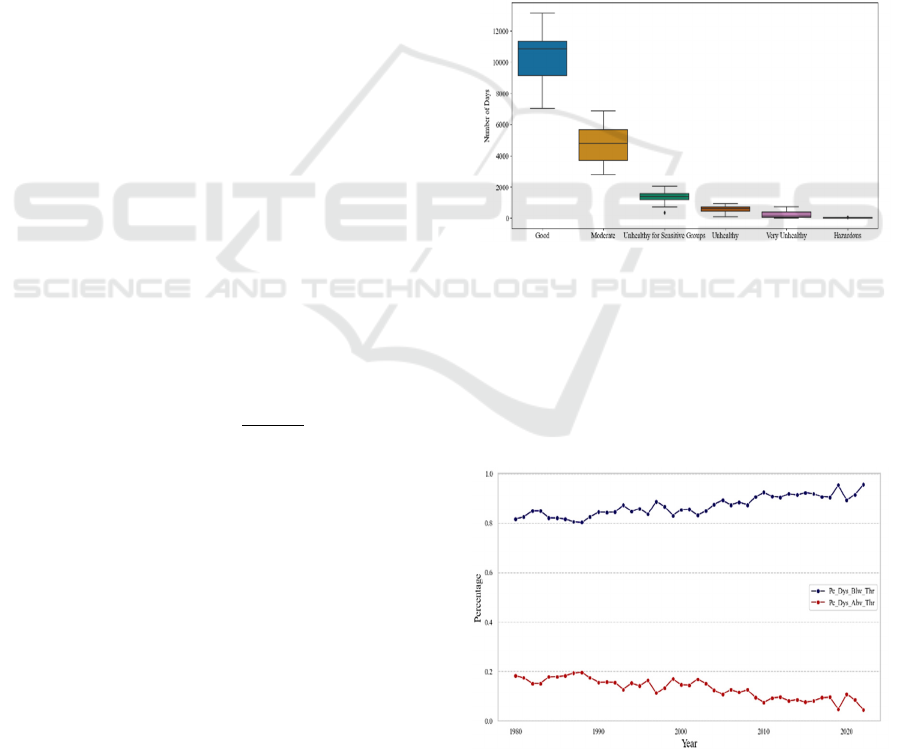
air quality management strategies. Initially, box plots

were drawn to depict the distribution of days across

six air quality categories: good, moderate, unhealthy

for sensitive groups, unhealthy, very unhealthy, and

hazardous, as shown in Fig.1.

From Figure 1, it can be observed that 'Good

Days' and 'Moderate Days' are prevalent, indicating

that in many years, the majority of days in California

have good air quality, signifying clean air for

residents most of the time. However, the occurrence

of days categorized as unhealthy for sensitive groups,

unhealthy, very unhealthy, and hazardous, although

fewer, still indicates periods of deteriorating air

quality that warrant attention.

Figure 1: Distribution of Air Quality Category Days

(Picture credit: Original).

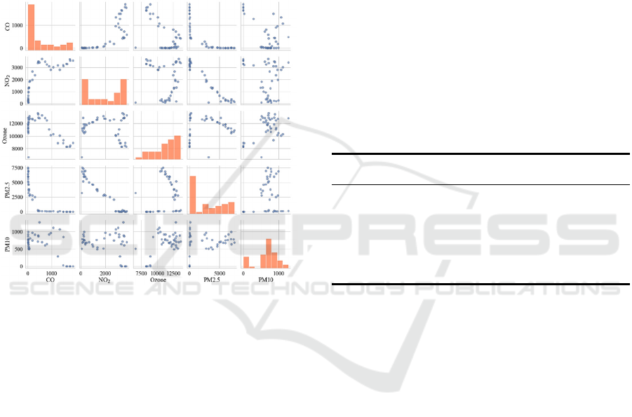
To further explore the trends in air quality

changes, related line plots were made, as shown in

Figure 2. Pc_Dys_Blw_Thr represents the percentage

of days with air quality below the moderate threshold,

while Pc_Dys_Abv_Thr represents the percentage of

days above the moderate threshold.

Figure 2: Trends in Air Quality Changes (Photo/Picture

credit: Original).

ICDSE 2024 - International Conference on Data Science and Engineering

From Figure 2, it is evident that over time, the

percentage of days with air quality below the

moderate threshold generally exhibits an upward

trend, while the percentage of days above the

threshold shows the opposite trend. This may reflect

the combined impact of various factors such as

environmental policies, urbanization, population

growth, and climate change.

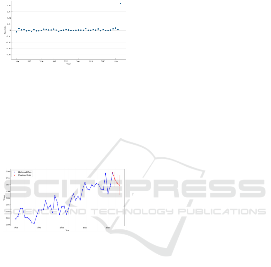
Finally, as illustrated in Figure 3, the matrix

scatter plot displays the distribution of days for five

major pollutants in California each year and the

relationships between different pollutants.

Figure 3: Matrix Scatter Plot of Major Pollutant Days

(Photo/Picture credit: Original).

The diagonal histograms reveal certain pollutants,

such as PM2.5 and PM10, have a broad range of

distribution, indicating significant variability in the

number of days they affect each year. The scatter

plots indicate some linear correlations between the

days of certain pollutants, suggesting that the

interactive effects between these pollutants need to be

considered in subsequent regression analyses.

3.2 Exploration of Influencing Factors

Based on the characteristics of the data, a preliminary

correlation between various pollutants, estimated

population, and Pc_Dys_Blw_Thr can be observed,

along with certain interactions among different

pollutants. Consequently, this study has decided to

establish a multiple linear regression model to

investigate the functional relationship between

Pc_Dys_Blw_Thr and various pollutants as well as

estimated population values. After several trials and

to avoid the issue of heteroscedasticity, this study has

employed robust standard errors (Croux et al. 2004)

during the regression process. The standardized

regression results obtained through the STATA

software are as follows:

𝑦3.384𝑥



0.121𝑥



0.573𝑥



0.392𝑥



𝑥



0.302𝑥



𝑥



(5)

where 𝑦 is the dependent variable

Pc_Dys_Blw_Thr, 𝑥



, 𝑥



, 𝑥



, 𝑥



and 𝑥



represent

Days CO, Days Ozone, Days PM2.5, Days NO2, and

Days PM10, respectively.

For the linear regression, the model achieved a

Prob > F value of 0.000 < 0.05, indicating that at a

95% confidence level, the model passes the joint

significance test. The adjusted R-squared is 0.9072,

demonstrating the model's reliability in explaining the

variance in the dependent variable. The

corresponding regression coefficient tests are

presented in Table 2.

Table 2: Regression Coefficient Table.

Beta

Coef.

Robust

Std. Err.

t P > | t |

𝑥



-3.384 0.000 -3.87 0.000

***

𝑥



0.121 0.000 0.80 0.015

𝑥



-0.573 0.000 -2.01 0.001

***

𝑥



𝑥



-0.392 0.000 -4.01 0.000

***

𝑥



𝑥



-0.302 0.000 -2.05 0.001

***

cons 0.000 0.033 29.06 0.000

***

Note:

***

and

represent significance levels of 1%, 5% and

10%, respectively

At a 95% confidence level, all regression

coefficients and the constant term have p-values less

than 0.05, indicating that the null hypothesis is

rejected and the results have passed the significance

test. This signifies that the regression coefficients are

highly reliable. Building upon this, the study

produced a regression residual plot and conducted a

multicollinearity test using STATA software,

respectively shown in Figure 4 and Table 3.

Study on the Inﬂuencing Factors and Prediction of Air Quality in California Based on Multiple Linear Regression and Gaussian Process

Regression Models

Figure 4: Regression Residual Plot (Picture credit:

Original).

Table 3: Multicollinearity Test.

Variable VIF

𝑥



8.19

𝑥



7.55

𝑥



3.13

𝑥



𝑥



3.10

𝑥



𝑥



1.86

From Figure 4, it is observed that all residuals are

evenly distributed between -0.04 and 0.04, indicating

a minimal heteroscedastic effect in the model. Table

3 shows that the highest Variance Inflation Factor

(VIF) is less than 10, suggesting that the regression

equation does not suffer from severe multicollinearity

issues.

In investigating the factors affecting air quality in

California, standardized regression results revealed a

significant negative correlation between the number

of days of major pollutants like CO and PM2.5 and

the percentage of days with air quality below the

moderate threshold. Specifically, CO exhibited the

most substantial negative impact on air quality,

underscoring the importance of reducing emissions of

these pollutants to improve air quality.

Regarding the positive correlation between ozone

and air quality, although the impact is relatively

small, it might reflect that under conditions of good

air quality, favorable sunlight and temperature

conditions are conducive to photochemical reactions

in the air, which may increase the concentration of

ground-level ozone, thereby affecting the ozone

levels in the air to a certain extent (Yu et al. 2021).

The significance of interaction terms further

emphasizes the impact of interactions between

different pollutants on air quality. Notably, the

negative coefficient for the interaction between

PM2.5 and NO2 suggests that these pollutants may

partially offset each other's impact when present

together, reducing their individual negative effects on

air quality. This is consistent with the visualization of

scatter plots where PM2.5 and NO2, as major

pollutants, show negative correlations. As such, the

air quality management strategies should account for

cross-impacts of pollutants instead of controlling

them individually. For instance, lower concentrations

of PM2.5 or nitrogen dioxide could improve air

quality in isolation; however, the consideration of

interactions between pollutants even on high

pollution days is more effective for preventing

deterioration of the air quality.

3.3 Forecasts of Air Quality Trends

In the field of machine learning, the generalization

ability of a model is particularly important when

making predictions on data. To better measure the

model's generalization ability and predictive

performance, this experiment divides the dataset into

a training set and a test set with an 8:2 ratio. The

training set is used to train the established model,

while the test set is used to evaluate the model's

generalization ability. As the predictive variable

(Pc_Dys_Blw_Thr) in this study is continuous, a

quadratic rational Gaussian process regression model

is adopted. Commonly used evaluation metrics in

regression models include Root Mean Square Error

(RMSE), Mean Absolute Error (MAE), Mean

Squared Error (MSE), and Coefficient of

Determination (𝑅



) (Tatachar 2021).

After multiple trials, the evaluation metrics for the

test set of the trained model, Series Fitting Plot, and

Residual Plot were obtained, respectively shown in

TABLE 4, Figure 5, and Figure 6.

Table 4: Test Set Evaluation Metrics.

RMSE MSE MAE

𝑹

𝟐

0.0061 3.668e-04 0.0018 0.97

Figure 5: Series Fitting Plot (Picture credit: Original).

ICDSE 2024 - International Conference on Data Science and Engineering

Figure 6: Residual Plot (Picture credit: Original).

The observations from the graphs and tables

indicate that the test set error is quite small, and the

coefficient of determination is high. Figure 5 shows

good fitting, and the scatter distribution in the residual

plot is relatively uniform, suggesting that the model

has strong generalization ability and can be used to

predict the future trend of Pc_Dys_Blw_Thr.

Utilizing the trained quadratic rational Gaussian

process regression model, predictions for the

percentage of days below the moderate threshold

from 2023 to 2025 were made, and the results are

presented in Figure 7.

Figure 7: Three-Year Prediction Plot for Pc_Dys_Blw_Thr

(Picture credit: Original).

Through the analysis of historical data from

California from 1980 to 2022, the study has found

that despite annual fluctuations, the overall level of

air quality in California has been gradually improving

over time. This improvement can be attributed to

increasingly stringent environmental policies,

technological advancements, and a heightened public

awareness of the importance of clean air over the past

few decades.

In particular, air quality is predicted to fall very

rapidly during 2020–2022, which was one of the main

results achieved by this research work. It was a time

when the epidemic of COVID-19 spread all over the

world, which resulted in unprecedented lockdown

measures across borders and regions such as

California (Johnson et al. 2021). The active measures

about restrictions of traffic flows, industrial activity

suspension, and other SWMs had a direct influence

on pollutant emission decrease that provided marked

precipitous air quality improvement in the short run.

Nevertheless, since the epidemic has gradually

subsided and economic activities come back to life by

2023-2025 years as predicted in this model air quality

index has lowered. This entails that a lack of constant

control and amelioration measures may result in

further human activities becoming instrumental in

poor air quality performance.

Accordingly, while the occurrence of a pandemic

may result in short-term improvements as regards air

quality management and improvement California will

need to continue focusing on such aspects. This

entails implementing sustainable pollution control

policies, increasing the adoption of renewable energy,

and reducing emissions from environmentally

unfriendly forms of transport as a measure to educate

citizens on conserving nature. Second, controlling

and evaluating the patterns as well as those that

influence air quality are needed for developing

policies and fine-tuning them to ensure timely

delivery through appropriate measures. With these

measures, air quality improvement becomes

sustainable in ensuring good public health and

maintaining a healthy environment.

In this holistic and proactive research approach,

the changes in air quality in California can be fully

understood and anticipated for a chance to stage

scientifically effective policies on environmental

measures as well as strategies for managing quality.

4 CONCLUSION

This research systematically assesses the air quality

data in California from more than four decades of

measurements and identifies the association between

pollutant emissions, and interactive effects among

various pollutants' impact on ambient air equality. By

developing accurate data analysis and modelling, the

research points out some short-term air quality

improvements during COVID-19 while forecasting

potential risks in post-recovery. These results

underscore the importance of ongoing surveillance

and necessary policy changes that are critical inputs

for public health, as well as environmental

stewardship. The results of the study also contribute

to science by offering a scientific argument for

strengthening air quality management techniques.

California and worldwide, thereby promoting

research-related areas. The research concludes that

people should take more note of the eventual effects

derived from an altered composition of pollution

Study on the Inﬂuencing Factors and Prediction of Air Quality in California Based on Multiple Linear Regression and Gaussian Process

Regression Models

sources, technological innovations preferences, and

policy modifications caused by altering climate

change on both air quality management systems as

well as health measures. By developing new and

innovative ideas, people can deal better with

challenges regarding natural environments to protect

average human health to assure the future of the

Earth.

REFERENCES

A. V. Tatachar, International Journal of Innovative

Technology and Exploring Engineering, 853-860

(2021).

A. Y. Bigazzi and M. Rouleau, Journal of Transport &

Health 7, 111-124 (2017).

C. Croux, G. Dhaene and D. Hoorelbeke, CES-Discussion

paper series (DPS) 16, 1-20 (2004).

D. Zhu, C. Cai, T. Yang and X. Zhou, Big data and

cognitive computing 2(1), 5 (2018).

I. Manisalidis, E. Stavropoulou, A. Stavropoulos and E.

Bezirtzoglou, Frontiers in public health 8, 14 (2020).

J. Liu, L. P. Clark, M. J. Bechle, A. Hajat, S. Y. Kim, A. L.

Robinson, et al., Environmental Health Perspectives

129(12), 127005 (2021).

K. A. Johnson, N. O. Burghardt and E. C. Tang, Sexually

Transmitted Diseases, 606-613 (2021).

M. Arfanuzzaman and B. Dahiya, Growth and Change

50(2), 725-744 (2019).

M. T. Lei, J. Monjardino, L. Mendes, D. Gonçalves and F.

Ferreira, Air Quality, Atmosphere & Health 12, 1049-

1057 (2019).

N. H. A. Rahman, M. H. Lee, Suhartono and M. T. Latif,

Quality & Quantity 49, 2633-2647 (2015).

O. Laurent, J. Hu, L. Li, M. J. Kleeman, S. M. Bartell, M.

Cockburn, L. Escobedo and J. Wu, Environment

International, Volumes 92, 471-477 (2016).

R. Yu, Y. Lin and J. Zou, Atmosphere 12(12), 1675 (2021).

X. Zhang, L. Han, H. Wei, X. Tan, W. Zhou, W. Li and Y.

Qian, Journal of Cleaner Production, 346 (2022).

Z. Yang and J. Wang, Environmental research 158, 105-117

(2017).

ICDSE 2024 - International Conference on Data Science and Engineering