Code Obfuscation Classification Using Singular Value Decomposition
on Grayscale Image Representations
Sebastian Raubitzek
2
, Sebastian Schrittwieser
1
, Caroline Lawitschka
1
, Kevin Mallinger
1
,
Andreas Ekelhart
2
and Edgar Weippl
2
1
Christian Doppler Laboratory for Assurance and Transparency in Software Protection,
Faculty of Computer Science, University of Vienna, Austria
2
SBA Research, Vienna, Austria
Keywords:
Code Obfuscation, Visual Analysis, Singular Value Decomposition.
Abstract:
In the ever-evolving world of cybersecurity, malware code hidden through code obfuscation is a key challenge
for detection systems. This research explores how to identify and analyze these obfuscations by turning binary
code into grayscale images, avoiding traditional code analysis methods that obfuscations might disrupt. We
convert the bytes of binary code to grayscale values and use singular value decomposition (SVD) to uncover
patterns that different obfuscation techniques create in the images. This method helps us see if specific obfus-
cation approaches cause unique patterns in the binary data, allowing us to classify them accurately. We apply
this technique to improve malware obfuscation detection and help software developers choose obfuscation
methods that are harder to spot. The main achievements of this study include developing a dependable system
for classifying obfuscated code, a detailed evaluation of how obfuscations affect binary structure and visual
representations thereof, and insights into using visual analysis for structural code analysis.
1 INTRODUCTION
In the world of cybersecurity, malware is a constant
and evolving threat. One of the most common meth-
ods malware developers use to evade detection by
anti-virus software is code obfuscation such as pack-
ing or virtualization. These code transformations ob-
scure the true purpose and functionality of the code,
making it much more challenging to analyze and clas-
sify. Therefore, it is essential for the effectiveness of
malware analysis on a large scale to undo them (de-
obfuscation) or use code analysis methods that are
least affected by a particular obfuscation or tools that
are able to handle that obfuscation best in order to
reveal the hidden functionality behind them. For tar-
geted analysis, it is, thus, important to first identify the
particular obfuscation techniques used as targeted de-
obfuscation methodologies often exist. Reliable de-
tection of obfuscation types is therefore of great im-
portance, and it is crucial to perform this detection
without relying on syntactic-based code analysis tech-
niques such as disassembling, which may be limited
in their correctness and coverage because of the ap-
plied obfuscation techniques.
On the other hand, code obfuscation is also an
essential instrument for protecting benign software.
It helps to prevent the unauthorized use of software,
for example, the removal of copy protection measures
or human-assisted reverse engineering. Software de-
velopers often want to know which obfuscation tech-
niques change the structure of the binary code the
least and are, therefore, the most difficult to detect.
In this work, a methodology frequently described
in the literature on malware detection is applied to
code obfuscation: the visual representation and anal-
ysis of binary code in the form of grayscale images.
Here, the individual bytes of binary code are inter-
preted as greyscale values and displayed as a two-
dimensional image. While such visual techniques
have so far mainly been used to recognize patterns
characteristic of certain malware families, we are in-
vestigating which specific patterns are generated in
the binary code by different obfuscation techniques.
Based on the hypothesis that obfuscation tech-
niques that modify similar aspects of the code, such
as its control flow or data structures, also generate
similar structural patterns in the binary code, we
evaluate whether these patterns can be reliably
Raubitzek, S., Schrittwieser, S., Lawitschka, C., Mallinger, K., Ekelhart, A. and Weippl, E.
Code Obfuscation Classification Using Singular Value Decomposition on Grayscale Image Representations.
DOI: 10.5220/0012856600003767
Paper published under CC license (CC BY-NC-ND 4.0)
In Proceedings of the 21st International Conference on Security and Cryptography (SECRYPT 2024), pages 323-333
ISBN: 978-989-758-709-2; ISSN: 2184-7711
Proceedings Copyright © 2024 by SCITEPRESS – Science and Technology Publications, Lda.
323

classified.
Our main contributions are:
• We present a novel code obfuscation classification
methodology using singular value decomposition
on grayscale image representations of the binary
code.
• Based on a large-scale evaluation with 3870 bi-
nary files, we demonstrate the feasibility of our
approach and interpret the results based on feature
importance.
The remainder of this paper is as follows: In Sec-
tion 2, we present related work. Section 3 introduces
our SVD-based machine learning classification ap-
proach, while in Section 4, we describe and discuss
the results of our experiments. Finally, Section 5 con-
cludes the paper. Further, we provide a corresponding
GitHub repository for reproducing our results
1
.
2 RELATED WORK
The visual representation of binary code has a long
tradition, particularly in malware detection and anal-
ysis. Early in the field, Nataraj et al. (2011) es-
tablished foundational work on malware detection
through binary visualization, introducing a method
for automatic classification based on traditional image
processing techniques. Their approach first demon-
strated that visual patterns derived from binaries can
be used to effectively differentiate between different
malware families.
Specifically, deep learning approaches for image-
based malware classification (Conti et al., 2022; Rus-
tam et al., 2023; Guo et al., 2023; Sharma et al., 2022;
Deng et al., 2023; Kumar et al., 2024) have gained in
popularity over the years.
Kalash et al. (2018), for example, proposed a
Convoluted Neural Network (CNN) based approach
for malware classification, diverging from traditional
but shallow learning algorithms such as Support Vec-
tor Machines (SVMs). They transformed malware bi-
naries into grayscale images, which were then used
to train a CNN, achieving better than state of the art
performance in 2018, with an accuracy of 98.52%
and 99.97% on the Malimg and Microsoft malware
datasets, respectively.
Ni et al. (2018) introduced the MCSC algo-
rithm, which employs feature extraction from disas-
sembled malware codes using SimHash, followed by
1
https://github.com/Raubkatz/Visual Obfuscation
Identification
their conversion into images for CNN-based classifi-
cation. This approach achieved an average accuracy
of 98.86% across a dataset of 10,805 samples.
Pinhero et al. (2021) also conducted an ex-
perimental approach in malware classification us-
ing CNN. Here, the input files were visualized as
grayscale, RGB as well as Markov images with varied
image dimensions (32 x 32, 64 x 64, 128 x 128, 256
x 256). Additionally, Gabor filters were applied to all
three types of images for feature extraction. The au-
thors experimented with twelve different neural net-
work architectures for classification. The proposed
approach produced an F-measure of 99.97%
Also, obfuscation detection methodologies based
on visual representations of binaries were discussed in
the literature. O’Shaughnessy and Sheridan (2022)
used a combination of dynamic as well as static
analysis while differentiation between obfuscated and
non-obfuscated samples. They utilized space-filling
curves to convert non-obfuscated malware executa-
bles and obfuscated sample process dumps into im-
ages. Classifiers were then trained on features ex-
tracted from these images using Local Binary Pat-
terns, Gabor filters and the Histogram of Oriented
Gradients. The dataset included 13,599 obfuscated
and non-obfuscated malware samples and produced
an accuracy of 97.6%.
In 2021, Parker et al. (2021) addressed the chal-
lenge of analyzing obfuscated code by proposing an
approach that involves visualizing obfuscated code bi-
naries into grayscale images. These images are then
resized to 64 x 64 pixels and subsequently used to
train a CNN for classification. The classification re-
sulted in F1-scores between 90% and 100% across all
tests.
Quist and Liebrock (2009) utilized the Ether hy-
pervisor framework to monitor program execution,
which was then processed and visually presented to
aid in understanding a program’s flow and structure.
By determining the optimal time to dump the current
state of the running program, this approach is capable
of circumventing any packer or obfuscation within the
executable. By creating visual maps of the program’s
execution and highlighting frequently executed areas,
this approach can indicate unpacking routines and ob-
fuscated code segments.
As the use of machine learning for image-based
malware classification became more popular, there
was also an increase of interest in potential coun-
termeasures as shown by Park et al. (2019).
They proposed a novel approach generating adver-
sarial malware examples that employs a dynamic
programming-based insertion algorithm to obfuscate
the .text section of a binary, maintaining the origi-
SECRYPT 2024 - 21st International Conference on Security and Cryptography
324

nal functionality while inducing high misclassifica-
tion rates in both white-box and black-box settings.
3 APPROACH
Our approach consists of five consecutive steps, de-
picted in Figure 1. The first step involves the cura-
tion of a collection of binaries used for analysis and
to train our models, as described in Section 3.1.
Second, we transform these binaries into 2D
grayscale images to obtain a matrix representation of
our binary code, Section 3.2.
Third, we use singular value decomposition to ob-
tain the spectrum of singular values for each matrix,
which we then use to construct a feature vector using
these complexity metrics, as detailed in Section 3.3.
Fourth, we train a tree-based classifier using this
dataset to identify different obfuscation methods and
non-obfuscated binary code, as explained in Sec-
tion 3.4.
Fifth, we use this approach to derive knowledge
on both the classification process and the different
complexity metrics based on the estimated obfusca-
tions and non-obfuscated binaries, discussed in Sec-
tion 4.
3.1 Dataset Generation
We created our own labeled dataset for model
generation by treating 190 programs in C source
code with various obfuscation configurations and
then compiling them into binary code using different
compiler configurations. The input programs were
divided into two categories: First, we composed a
set of 85 single-function programs such as hashing
or sorting algorithms. We both included samples
from the obfuscation dataset by Banescu et al. (2015)
and self-written algorithms. Second, we extended
the dataset with programs from the GNU Core
Utilities collection. We then created non-obfuscated
binaries from all source files using various compiler
configurations: Each source code was compiled
with both gcc and clang on four optimization levels
(-O0 to -O3), and additional binaries were created
with the special-purpose compilers TinyCC (both in
latest release version 0.9.27 from 2017 and well as
the head version from its development branch) and
Tendra. For the obfuscated binaries, we used the
state-of-the-art source-to-source obfuscator Tigress.
Since Tigress only accepts single-file C programs, we
preprocessed all samples from the Core Utilities with
the merge function of CIL
2
. Based on the hypothesis
that obfuscations that transform similar structural
properties of the program code also generate similar
visual representations in the binary, we classified
the applied obfuscations into two categories (Schrit-
twieser et al., 2016):
Control flow obfuscations change the control flow of
a program. We used two techniques that work on dif-
ferent levels:
• The flatten technique removes the structured flow
of basic blocks within a function by inserting a
central dispatcher that is jumped to after executing
a basic block.
• With the split technique, functions are split up
and parts of the functionality is outsourced to a
new functions. This obfuscation modifies the pro-
gram’s call graph.
Dynamic obfuscations transform the program in such
a way that the code executed at runtime is no longer
explicitly stored in the binary code but is recon-
structed at runtime. We applied the following two
techniques to our samples:
• The virtualization technique transforms a func-
tion into an interpreter whose randomly generated
bytecode was created specifically for this func-
tion. At runtime, this bytecode is interpreted and
converted into the actual machine code which is
then executed.
• With the JIT technique, intermediate code in the
binary is compiled and executed just-in-time at
runtime.
It is important to emphasize that in practical soft-
ware protection scenarios, obfuscations should not
be used in isolation but always in combination with
other techniques (obfuscation layering). In this work,
however, we aim to analyze the effects of individual
techniques on the binary code structure in isolation.
Therefore, we treated each protected sample with a
single obfuscation.
In total, we used 35 different build and obfusca-
tion configurations (gcc and clang, each in four opti-
mization levels, Tendra, two versions of TinyCC, and
four different Tigress obfuscations, each in four opti-
mization levels). We conducted a simple functionality
check for each binary and excluded broken samples.
In total, we generated 3870 fully functional binaries,
which comprise the dataset for this work.
2
http://cil-project.github.io/cil/doc/html/cil/merger.html
Code Obfuscation Classification Using Singular Value Decomposition on Grayscale Image Representations
325

Figure 1: Developed Pipeline Overview: This figure illustrates our data processing and analysis pipeline. Starting from binary
code, we transform it into a grayscale image. Subsequently, we calculate SVD complexity metrics from this grayscale image.
These metrics are then used as an input vector for our ExtraTrees Machine Learning classification approach, which enables
us to classify different obfuscation methods versus non-obfuscated binaries.
3.2 Grayscale Image Representation
We start by converting raw binary data into a 1-
dimensional array of bytes, where each byte repre-
sents a pixel value in a grayscale image. We then
check if the length of this array is sufficient to fill a
2-dimensional image. If the array is too short, we pad
it with zeros at the end to ensure it has enough data
to form a complete image. Finally, we reshape this
array into a 2-dimensional array that represents the
grayscale image, with each element corresponding to
a pixel’s intensity (0 to 255).
3.3 Feature Extraction
Given our transformation of binary code into
grayscale images, i.e., 2D matrices, we can utilize a
variety of tools to extract features from these matrices.
Before diving into the description of our employed
metrics, we acknowledge that there is a vast array of
complexity metrics available that we did not consider
in this article and which might be addressed in future
research. Examples include classic complexity met-
rics applicable to binary code, such as Lempel-Ziv
complexity, other basic complexities of binary code,
and different matrix complexities similar to fractal di-
mensions, where one considers the sort of density of
partitions of matrices.
In this work, we employ complexity metrics based
on a singular value decomposition (SVD) of a matrix
and aim to extract relative information from the corre-
sponding spectrum of singular values. Here, relative
implies that we do not consider the absolute number
of singular values or the exact sizes of the matrices,
ensuring our approach is agnostic of the size and pre-
cise dimensions of the matrix. This methodology al-
lows us to analyze, for example, the relative decay of
the obtained spectrum of singular values. Interpreting
these complexities via singular value decomposition
suggests that the spectrum characterizes the strength
of certain base vectors needed to construct a matrix.
This can also be used inversely to compress a matrix
or an image’s information, as only the base vectors
with large enough singular values are required to char-
acterize the information of an image (Prasantha et al.,
2007).
For our use case, this means our spectrum of
singular values, e.g., of a transformed binary file,
characterizes how fine-grained the binary is and/or
how dense it is, consequently indicating how many
of these base vectors are needed to span the matrix.
Thus, the relative information of this spectrum of sin-
gular values carries significant insights into the struc-
ture, density
3
and overall complexity of an analyzed
matrix.
Singular Value Decomposition (SVD). is used as a
tool to reduce the dimensionality of data by collapsing
complex, high-dimensional data arrays into a vector
of values, i.e., the spectrum of singular values. Given
a matrix A, SVD is performed by the following fac-
torization:
A = U ΣU
†
(1)
where:
• U is an orthogonal matrix.
• Σ is a diagonal matrix with real, non-negative sin-
gular values, σ
i
, which are ordered from largest
to smallest: σ
i
= [σ
0
, σ
1
, σ
2
, ..., σ
p
], where
p = min(m, n), i.e. the rank of the regarded ma-
trix.
3
Note that we use these terms loosely without a strict
definition, to provide an abstract understanding of our fea-
ture space’s information.
SECRYPT 2024 - 21st International Conference on Security and Cryptography
326

• U
†
is the conjugate transpose of U.
We then also also normalize the singular values, rep-
resented as
¯
σ
i
:
¯
σ
i
=
σ
i
∑
p
j=1
σ
j
(2)
To extract a set of features from our grayscale
images we employed the following set of SVD-based
complexity metrics:
1. SVD-Entropy:
Entropy, introduced by Claude Shannon (Shan-
non, 1948) quantifies the amount of unpredictabil-
ity or information content in a dataset. The corre-
sponding formula calculates entropy by summing
the product of each unique value’s probability (p
i
)
and the logarithm of that probability. The formula
can be applied with different logarithmic bases b,
such as b = 2 (bits), b = e (nats, with e - Euler’s
number), or b = 10 (digits) and has the following
expression:
H
Shannon
= −p
i
m
∑
i
log
b
(p
i
) (3)
Entropy applied on the Singular Value Decompo-
sition values quantifies randomness in the distri-
bution of singular values of a matrix. A high en-
tropy value indicates a higher degree of irregular-
ity among the singular values, Applied to the SVD
values, Shannon’s Entropy is adapted such that:
H
SV D
= −
r
∑
i=1
¯
σ
i
log
2
¯
σ
i
(4)
This concept originates from the study of medical
time series data, but applies to spectra of singu-
lar values of matrices in general,(Roberts et al.,
1999).
2. Relative Decay of Singular Values:
Relative Decay measures the rate of reduction in
singular values from the largest to the smallest,
effectively capturing the slope of descending sin-
gular values. It is mathematically defined as:
D
rel
(A) =
σ
i
σ
i+1
(5)
where σ
i
and σ
i+1
are consecutive singular val-
ues of matrix A. This ratio indicates how quickly
the singular values decrease, where a rapid decay
suggests that the matrix can be approximated ef-
fectively by a lower-dimensional subspace. Such
an attribute is advantageous in fields like signal
processing and data compression. Conversely, a
slow decay implies a higher complexity within
the matrix, indicating a more uniform distribution
of information across its dimensions. This met-
ric is particularly valuable in systems analysis and
model reduction, where it correlates with the effi-
ciency of approximation methods (Antoulas et al.,
2002).
3. Singular Spectral Radius:
The spectral radius of a matrix is the maximum of
the absolute values of its singular values:
ρ(A) = max
i
|σ
i
| (6)
This metric is known to characterize large random
matrices as pointed out by the work of Alt, Erd
˝
os,
and Kr
¨
uger (Alt et al., 2021).
4. SVD-Energy:
Singular Value Decomposition (SVD) Energy
(or Energy Ratio) is a metric derived from the
singular values of a matrix, sort of depicting
the ’energy’ contained within the dominant val-
ues(Razafindradina et al., 2017). It is calculated
as the sum of the squares of the dominant singu-
lar values normalized by the total energy, formally
expressed as:
E
SVD
=
∑
k
i=1
σ
2
i
∑
p
i=1
σ
2
i
, (7)
where we chose k = 3. High SVD Energy val-
ues suggest that a few singular values dominate
the energy spectrum, indicating a matrix with
pronounced principal components, which can be
critical for applications such as image compres-
sion and noise reduction. Conversely, a lower
SVD Energy indicates a more uniform distribu-
tion of singular values, reflective of a matrix with
complex, evenly distributed features, beneficial in
fields requiring detailed, non-reductive data anal-
ysis, such as high-dimensional data visualization
and intricate pattern recognition.
5. Fisher’s Information:
We perform a calculation similar to the previous
one for SVD-entropy to obtain Fisher’s informa-
tion from the spectrum of singular values. How-
ever, contrary to SVD entropy, Fisher’s informa-
tion depicts the difference between the individual
singular values rather than employing Shannon’s
entropy for analysis. Fisher Information measures
the amount of information that the singular val-
ues of a matrix convey about the system it rep-
resents. This is, however, not as Fisher’s infor-
mation was originally developed (Fisher, 1922),
but a more pragmatic adapted formulation as used
Code Obfuscation Classification Using Singular Value Decomposition on Grayscale Image Representations
327

to analyze physiological signals (Makowski et al.,
2021). Again, we make use of the fact, that we
can calculate singular values of our matrices and
analyze the spectrum of these accordingly:
I
Fisher
=
r−1
∑
i=1
[
¯
σ
i+1
−
¯
σ
i
]
2
¯
σ
i
(8)
6. Condition Number:
The condition number of a matrix is calculated as
the ratio of the maximum to the minimum singular
value:
κ(A) =
max(σ)
min(σ)
(9)
where σ represents the singular values of matrix
A. This measure is particularly crucial in analyz-
ing random matrices, common in stochastic mod-
eling and data simulations, where it assesses the
robustness of numerical algorithms and the relia-
bility of modeled systems (Edelman, 1988). Here,
we introduced a threshold for the lower singular
values to avoid a division by zero or very small
numbers; this threshold was chosen to be 10
−6
,
i.e., no values below this were considered in the
calculation of the condition number.
These tools served to extract features from our gray-
scale images to build our feature vectors used as the
input for our machine learning model in the follow-
ing ML classification approach. I.e., for each sample
(grayscale image), we get a vector consisting of the
above six values/metrics.
3.4 Machine Learning Classification
In this study, we employed an ensemble learning
method known as the Extra Trees (Extremely Ran-
domized Trees) classifier, originally introduced by
Geurts et al. (2006). We further split the data in an
80/20 ratio; training the data on 80% of the origi-
nal data and afterwards evaluating the models perfor-
mance on the remaining 20% of the data. To optimize
the hyperparameters of the Extra Trees classifier, we
utilized Bayesian Optimization with 5-fold Cross Val-
idation. Before training the model, we addressed the
class imbalance issue in our dataset by implement-
ing the ADASYN (Adaptive Synthetic Sampling) ap-
proach (He et al., 2008). This technique generates
synthetic samples from the minority class, thereby
creating a more balanced dataset and improving the
generalizability of our model. Further, ADASYN
was applied to the training data only. We evaluated
our models using four classification metrics that are
part of scikit-learn (Pedregosa et al., 2011): accu-
racy, precision, recall, and F1-score. The training
and cross-validation were performed using accuracy
as the scoring metric. Further, we also employed
feature-importance analysis, which is part of scikit-
learn for tree-based classifiers, to derive knowledge
on which complexity metric depicts our classification
best, i.e., has the biggest influence on the outcome.
All machine learning and analysis were performed
using Python.
4 RESULTS AND DISCUSSION
We present different levels of detail for our classifica-
tion approach, i.e., we start by classifying if a program
was obfuscated or not and further add more details un-
til we end up with a selection of differently obfuscated
and compiled programs. This approach allows us to
show and discuss different aspects of the problem rel-
evant in varying use-cases which we will discuss in
the following.
Overall, we discuss four different classification
approaches and the results thereof; note that we per-
formed all experiments on the same set of binary code
samples. Thus, our categories, presented in order of
descending groups, are:
• No Grouping
We used the data set as described in Sec-
tion 3.1 with varying obfuscation methods and
non-obfuscated code produced by different com-
pilers.
• Obfuscation Method vs. no Obfuscation
We grouped all non-obfuscated code samples into
one category.
• Category of Obfuscation vs. no Obfusca-
tion We grouped the four obfuscation methods
into three categories of obfuscations (see Sec-
tion 3.1. I.e. we grouped flatten and split into
TigressCFGObfuscation, and virtualize and
jit into TigressDynamicsObfuscation.
• Obfuscation vs. no Obfuscation
We reduced the problem to binary classifica-
tion to differ just between obfuscated and non-
obfuscated code.
All results for all groupings of our classification ap-
proach (according to Section 3.4) are presented in Ta-
ble 1. In the following, we discuss the different group-
ings and respective performances individually.
SECRYPT 2024 - 21st International Conference on Security and Cryptography
328

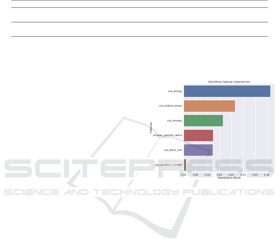
Table 1: Performance Metrics by Grouping.
Grouping Accuracy Precision Recall F1 Score
Best CV
Score
Obfuscation vs. No Obfuscation 0.9897 0.9897 0.9897 0.9897 0.9948
Obfuscation Categories vs. No
Obfuscation
0.8023 0.8075 0.8023 0.8037 0.8691
Obfuscation Types vs. No
Obfuscation
0.6718 0.6695 0.6718 0.6650 0.7718
No Grouping 0.6628 0.6607 0.6628 0.6598 0.8938
4.1 Grouping 1: Obfuscation or no
Obfuscation
We first discuss the simplest case: Can we identify
from our complexity spectrum if a binary is obfus-
cated?
Our results, as presented in Table 1, show that
we can very accurately identify if a binary was ob-
fuscated, i.e., close to 100%. All employed scores
and the result of the cross-validation indicate that
the grayscale depiction and, further, the complexity
thereof, depict the difference between obfuscated and
non-obfuscated binary code very well. When analyz-
ing which complexity contributes most to this clas-
sification, our feature importance analysis (Figure 2)
shows that SVD-energy is the most important feature
in this classification process. Therefore, the ratio of
the most significant singular values compared to the
full spectrum carries a lot of information about obfus-
cated and non-obfuscated code. This is supported by
the fact that the second most important feature is the
relative decay of singular values. This feature depicts
the difference of the largest to the smallest singular
values, as it is the slope of the descent of said val-
ues. Given our transformation into grayscale images,
this means that obfuscated and non-obfuscated bina-
ries are different in their fine-grainedness as SVD-
energy allows us to differentiate between more dis-
tributed and more peaking spectra of singular values
which then also refers to the binary. The difference
corresponds to some binaries having more ”islands”
of information than others. It is necessary to clar-
ify that we cannot precisely determine where these
islands occur or discuss their properties, as this would
require a more in-depth analysis of code complexity
and further ML explanatory and interpretability anal-
ysis.
Our results are important in the context of mal-
ware analysis, as we can very much always iden-
tify if the analyzed code is obfuscated and subse-
quently employ different strategies to analyze and
treat possible malicious code, even on a binary
level. According to these results, obfuscated malware
will always produce binaries with a different infor-
mation density/fine-grainedness than non-obfuscated
malware.
Figure 2: Feature Importances for: Obfuscated vs. Non-
Obfuscated Code.
4.2 Grouping 2: Non Obfuscated Code
vs. Different Categories of
Obfuscated Code
In this section, we group our obfuscated code
into two categories: CFG-based obfuscations
(TigressCFGObfuscation) and dynamic obfusca-
tions (TigressDynamicObfuscation). The results
are significantly worse than for the prior grouping.
That is, Accuracy, Precision, Recall, and F1 Score
are all around ≈ 0.80, whereas the best CV-Score is
at ≈ 0.87, as depicted in Table 1. However, if we take
a closer look at the corresponding confusion matrix
(Figure 3), we see that non-obfuscated code can
still be identified with high accuracy , whereas the
two categories for obfuscated code are still mistaken
for each other. This shows that although we can
identify if a code has been obfuscated, determining
which category of obfuscation it belongs to is more
challenging.
Code Obfuscation Classification Using Singular Value Decomposition on Grayscale Image Representations
329

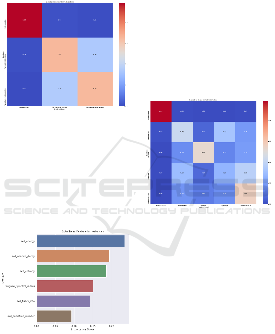
Figure 3: Confusion matrix for: Obfuscation Categories
vs. Non-Obfuscated
Similar to the previous discussion (Section 4.1),
the three most important complexity metrics are
SVD-energy, SVD-relative-decay, and SVD-entropy,
indicating that the fine-grainedness or density of the
code is most indicative of its obfuscation, as depicted
in Figure 4.
While determining which category of obfuscation
had been used to be difficult, we succeeded in cor-
rectly identifying obfuscated malware. Furthermore,
from a software protection standpoint, one would
choose an obfuscation category that can not be eas-
ily identified. In this particular case, both categories
are equally good for hiding the employed obfuscation.
Figure 4: Feature Importances for: Categories of Obfus-
cation vs. Non-Obfuscated Code.
4.3 Grouping 3
The next grouping examines the specific obfuscation
methods which were employed to our code, while
also comparing their classification to each other and
against non-obfuscated code.
While the results are worse than for the previous
case (Section 4.2), with all scores at ≈ 0.67, we ob-
serve that non-obfuscated code can be successfully
identified with very high accuracy, as shown in Fig-
ure 5. As for identifying obfuscation techniques,
TigressSplit is cloaked the best among other ob-
fuscation techniques, whereas TigressVirtualize
can be identified most accurately. As opposed to the
Figure 5: Confusion matrix for: Obfuscation Types vs.
Non-Obfuscated.
two previous classification tasks, SVD-energy is no
longer the most important feature; however, the top
three remain the same, albeit they switch places. This
once again supports our claims that the different dis-
tributions with respect to each other, i.e., how the sin-
gular value descent, depicts the type of binary the
best, as seen in Figure 6.
4.4 No Grouping
The final grouping depicts our effort to classify not
only obfuscated vs. non-obfuscated code but also
how we can identify obfuscated and non-obfuscated
code from different compilers. Our results are slightly
worse than for the previously discussed grouping
(Section 4.3), with accuracy, precision, F1 score, and
recall at ≈ 0.66. Our results depicted in Figure 7 show
that we can identify non-obfuscated code from dif-
ferent compilers with high accuracy. These results
also suggest that—taking into account the discussions
from Sections 4.1, 4.2, and 4.3—different compil-
SECRYPT 2024 - 21st International Conference on Security and Cryptography
330

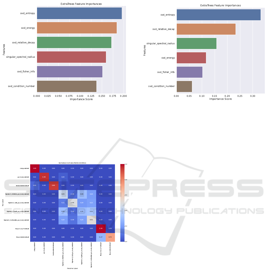
Figure 6: Feature Importances for: Obfuscation Method
vs. Non-Obfuscated Code.
ers and optimization levels have a strong signature in
terms of producing code with varying densities and a
signature fine-grainedness of information. This is also
supported by the corresponding feature importances,
shown in Figure 8.
Figure 7: Confusion matrix for: No Grouping. Everything
with tigress refers to an obfuscation technique.
However, regarding the feature importances, we
note that in this case, SVD entropy and SVD rela-
tive decay are still among the top three, with SVD en-
tropy reigning supreme, but SVD energy has dropped
to fourth place, as shown in Figure 8.
We conclude from this that although SVD energy
provides a lot of information with respect to identi-
fying if a code was obfuscated, the relative decay,
entropy, and spectral radius are more important for
differentiating between compilers and obfuscations.
An interesting result here is that for these classifica-
tions, the singular value spectral radius, which is just
Figure 8: Feature Importances for: No Grouping.
the absolute value of the maximum singular value, is
important. This further supports our claim that cer-
tain compilers and obfuscations produce ”islands of
information” (or not, conversely), as a very expres-
sive maximal singular value corresponds to dense el-
ements from the basis components of a matrix, i.e.,
one dense island, so to speak.
5 CONCLUSIONS
This article presents an approach to identify non-
obfuscated and differently obfuscated binary code.
Building on previous research, we use a transforma-
tion of binary code into grayscale images as discussed
in Section 3.2. Unlike other researchers who rely
on neural network architectures and synthetic code
bases for identifying obfuscated code (Parker et al.,
2021), we employ an interpretable, non-neural net-
work approach. Although neural networks generally
outperform other methods across various fields, they
are often viewed as non-interpretable black boxes.
Our approach emphasizes result interpretation and
generalizability, addressing the limitations of neural
networks, particularly convolutional neural networks,
whose fixed input frames pose challenges for varying
binary lengths. For our particular case, this means
that excessive missing bits are replaced with zeros,
and the convolutional layers impose upper boundaries
of input sizes that restrict generalizability. In contrast,
we use a tree-based boosting classifier combined with
complexity metrics that allow feature vector creation
independent of binary size, enhancing the model’s
adaptability and interpretability.
The curation of our code base also differentiates
our method from others, utilizing a collection of dif-
ferently sized, non-synthetic programs that perform
Code Obfuscation Classification Using Singular Value Decomposition on Grayscale Image Representations
331

various tasks, strengthening our approach’s robust-
ness.
Although our approach underperforms compared
to the results from Parker et al. (2021), which re-
port scores of approximately 0.99, our approach
achieves a score of ≈ 0.99 in identifying whether code
is obfuscated, with respect to accuracies. Despite
lower scores for identifying the particular obfuscation
method, we highlight our model’s superior general-
izability and nuanced classification. Using synthetic
code introduces bias, and the inability of CNNs to
handle arbitrary binary lengths implies that such mod-
els while enhancing certain features, do not generalize
well to real-world applications.
We can identify which features are crucial at each
classification level and interpret these features. For
example, different SVD metrics reveal the informa-
tion density and compressibility of the underlying bi-
nary. This not only allows us to discern that ob-
fuscated and non-obfuscated code differ primarily in
their SVD-energy but also provides insights for fu-
ture obfuscation techniques to avoid these character-
istics. Additionally, we observed that different com-
pilers produce signature binary densities, which are
identifiable in the classification process.
Ultimately, our approach demonstrates that the
generalizable, interpretable detection of obfuscation
techniques in real-life scenarios remains a challenge.
However, the ability of researchers to use these results
to circumvent traits that distinguish obfuscated from
non-obfuscated code suggests that this will be an ac-
tive area of ongoing research. Developments in ob-
fuscation techniques are likely to continue challeng-
ing older identification models and vice versa.
We encourage future research to focus on inter-
pretable, tree-based classifiers combined with com-
plexity metrics, as they offer interpretability and gen-
eralizability, contrary to overly specific and non-
interpretable neural network solutions that require
significant expertise to build and analyze and do not
allow for subsequent research on their inner workings.
ACKNOWLEDGEMENTS
The financial support by the Austrian Federal Min-
istry of Labour and Economy, the National Founda-
tion for Research, Technology and Development and
the Christian Doppler Research Association is grate-
fully acknowledged.
REFERENCES
Alt, J., Erd
˝
os, L., and Kr
¨
uger, T. (2021). Spectral radius of
random matrices with independent entries. Probabil-
ity and Mathematical Physics, 2(2):221–280.
Antoulas, A., Sorensen, D., and Zhou, Y. (2002). On the
decay rate of hankel singular values and related issues.
Systems & Control Letters, 46(5):323–342.
Banescu, S., Ochoa, M., and Pretschner, A. (2015).
A framework for measuring software obfuscation
resilience against automated attacks. In 2015
IEEE/ACM 1st International Workshop on Software
Protection, pages 45–51. IEEE.
Conti, M., Khandhar, S., and Vinod, P. (2022). A few-shot
malware classification approach for unknown fam-
ily recognition using malware feature visualization.
Computers & Security, 122:102887.
Deng, H., Guo, C., Shen, G., Cui, Y., and Ping, Y. (2023).
Mctvd: A malware classification method based on
three-channel visualization and deep learning. Com-
puters & Security, 126:103084.
Edelman, A. (1988). Eigenvalues and condition numbers of
random matrices. SIAM Journal on Matrix Analysis
and Applications, 9(4):543–560.
Fisher, R. A. (1922). On the mathematical foundations
of theoretical statistics. Philosophical Transactions
of the Royal Society of London. Series A, Contain-
ing Papers of a Mathematical or Physical Character,
222:309–368.
Geurts, P., Ernst, D., and Wehenkel, L. (2006). Extremely
randomized trees. Machine Learning, 63(1):3–42.
Guo, J., Xu, Y., Xu, W., Zhan, Y., Sun, Y., and Guo, S.
(2023). Mdenet: Multi-modal dual-embedding net-
works for malware open-set recognition.
He, H., Bai, Y., Garcia, E. A., and Li, S. (2008). Adasyn:
Adaptive synthetic sampling approach for imbalanced
learning. 2008 IEEE International Joint Conference
on Neural Networks (IEEE World Congress on Com-
putational Intelligence), pages 1322–1328.
Kalash, M., Rochan, M., Mohammed, N., Bruce, N. D.,
Wang, Y., and Iqbal, F. (2018). Malware classifica-
tion with deep convolutional neural networks. In 2018
9th IFIP international conference on new technolo-
gies, mobility and security (NTMS), pages 1–5. IEEE.
Kumar, S., Janet, B., and Neelakantan, S. (2024). Im-
cnn:intelligent malware classification using deep con-
volution neural networks as transfer learning and en-
semble learning in honeypot enabled organizational
network. Computer Communications, 216:16–33.
Makowski, D., Pham, T., Lau, Z. J., Brammer, J. C.,
Lespinasse, F., Pham, H., Sch
¨
olzel, C., and Chen, S.
H. A. (2021). NeuroKit2: A python toolbox for neu-
rophysiological signal processing. Behavior Research
Methods, 53(4):1689–1696.
Nataraj, L., Karthikeyan, S., Jacob, G., and Manjunath,
B. S. (2011). Malware images: visualization and auto-
matic classification. In Proceedings of the 8th interna-
tional symposium on visualization for cyber security,
pages 1–7.
SECRYPT 2024 - 21st International Conference on Security and Cryptography
332

Ni, S., Qian, Q., and Zhang, R. (2018). Malware identifi-
cation using visualization images and deep learning.
Computers & Security, 77:871–885.
O’Shaughnessy, S. and Sheridan, S. (2022). Image-
based malware classification hybrid framework based
on space-filling curves. Computers & Security,
116:102660.
Park, D., Khan, H., and Yener, B. (2019). Generation &
evaluation of adversarial examples for malware obfus-
cation. In 2019 18th IEEE International Conference
On Machine Learning And Applications (ICMLA),
pages 1283–1290. IEEE.
Parker, C., McDonald, J. T., and Damopoulos, D. (2021).
Machine learning classification of obfuscation using
image visualization. In SECRYPT, pages 854–859.
Pedregosa, F., Varoquaux, G., Gramfort, A., Michel, V.,
Thirion, B., Grisel, O., Blondel, M., Prettenhofer,
P., Weiss, R., Dubourg, V., Vanderplas, J., Passos,
A., Cournapeau, D., Brucher, M., Perrot, M., and
Duchesnay, E. (2011). Scikit-learn: Machine learning
in Python. Journal of Machine Learning Research,
12:2825–2830.
Pinhero, A., Anupama, M., Vinod, P., Visaggio, C. A.,
Aneesh, N., Abhijith, S., and AnanthaKrishnan, S.
(2021). Malware detection employed by visualiza-
tion and deep neural network. Computers & Security,
105:102247.
Prasantha, H., Shashidhara, H., and Balasubra-
manya Murthy, K. (2007). Image compression
using svd. In International Conference on Compu-
tational Intelligence and Multimedia Applications
(ICCIMA 2007), volume 3, pages 143–145.
Quist, D. A. and Liebrock, L. M. (2009). Visualizing com-
piled executables for malware analysis. In 2009 6th
International Workshop on Visualization for Cyber Se-
curity, pages 27–32.
Razafindradina, H. B., Randriamitantsoa, P. A., and
Razafindrakoto, N. R. (2017). Image compression
with SVD : A new quality metric based on energy ra-
tio. CoRR, abs/1701.06183.
Roberts, S. J., Penny, W., and Rezek, I. (1999). Temporal
and spatial complexity measures for electroencephalo-
gram based brain-computer interfacing. Medical &
Biological Engineering & Computing, 37(1):93–98.
Rustam, F., Ashraf, I., Jurcut, A. D., Bashir, A. K., and
Zikria, Y. B. (2023). Malware detection using im-
age representation of malware data and transfer learn-
ing. Journal of Parallel and Distributed Computing,
172:32–50.
Schrittwieser, S., Katzenbeisser, S., Kinder, J., Merzdovnik,
G., and Weippl, E. (2016). Protecting software
through obfuscation: Can it keep pace with progress
in code analysis? Acm computing surveys (csur),
49(1):1–37.
Shannon, C. E. (1948). A mathematical theory of communi-
cation. Bell System Technical Journal, 27(3):379–423.
Sharma, O., Sharma, A., and Kalia, A. (2022). Win-
dows and iot malware visualization and classification
with deep cnn and xception cnn using markov images.
Journal of Intelligent Information Systems, 60.
Code Obfuscation Classification Using Singular Value Decomposition on Grayscale Image Representations
333