Integrated Data-Driven Framework for Automatic Controller Tuning with

Setpoint Stabilization Through Reinforcement Learning

Babak Mohajer, Neelaksh Singh and Joram Liebeskind

BELIMO Automation AG, Brunnenbachstrasse 1, 8340 Hinwil, Switzerland

Keywords:

Simulation-Based Optimization, Automatic Controller Tuning, Bayesian Optimization, Time Series Clustering,

Online Learning, Reinforcement Learning, Setpoint Stabilization.

Abstract:

We introduce a three-stage framework for designing an optimal controller. First, we apply ofﬂine black-box

optimization algorithms to ﬁnd optimal controller parameters based on a heuristically chosen setpoint proﬁle

and a novel cost function for penalizing control signal oscillations and direction changes. Then, we leverage

cloud data to generate device-speciﬁc setpoint proﬁles and tune the controller parameters to perform well

on the device with respect to the same cost function. Finally, we train a control policy on top of the ofﬂine

tuned controller after deployment on device through an online learning algorithm to handle unseen setpoint

variations. A novel reward function encouraging setpoint stabilization is added for preventing destabilization

from coupling effects. Bayesian Optimization and Nelder-Mead methods are used for ofﬂine optimization, and

a state-of-the-art model free Reinforcement Learning algorithm namely Soft Actor-Critic is used for online

optimization. We validate our framework using a realistic HVAC hydraulic circuit simulation.

1 INTRODUCTION

Proportional integral derivative (PID) controllers are

at the core of a majority of control systems deployed

to this date owing to their simple design and robust

performance. However, they need adequate tuning to

perform effectively thus encouraging the development

of manual and automatic tuning strategies (Ziegler and

Nichols, 1993; Cohen and Coon, 2022; Garcia and

Morari, 1982;

Astr

om and H

agglund, 2004). With the

formulation of PID tuning as an optimization prob-

lem, modern optimization, data-driven, and machine-

learning (ML) based techniques saw widespread suc-

cess due to their proﬁciency in handling general non-

convex objective functions (Gaing, 2004; Ahmad et al.,

2021; Mok and Ahmad, 2022).

These data-driven techniques rely on repeated sim-

ulations and ofﬂine data collection. This leads to lim-

ited generalizability since the ofﬂine-data may not

capture all probable model operating points. For ex-

ample, in Heating, Ventilation, and Cooling (HVAC)

systems typical temperature setpoints vary with sea-

sons and geographical regions. Furthermore, in hier-

archical PID control systems, extremely non-linear in-

teractions between the subsystems cannot be captured

easily by ofﬂine tuning algorithms again necessitating

large-datasets which are expensive to collect. These

concerns led to development of data-driven control

algorithms which can adapt to changing conditions

online. The most notable methods are data-driven pre-

dictive control (Zhuang et al., 2023) and reinforcement

learning (RL) (Sutton and Barto, 2020).

RL is able to optimize general objectives without

any assumptions on convexity, differentiability, and

sparsity of the objective function. However, it relies

on learning by randomly exploring the feasible con-

trol input space which can destabilize the system if

deployed directly. Therefore, it is preferable to deploy

RL on top of a known suboptimal but stabilizing base

controller like PID as explored in (Solinas et al., 2024).

But if the underlying PID controller is poorly tuned,

the overall system will continue to behave poorly until

RL learns to take optimal actions, which takes quite

some time in practice due to model free RL’s low sam-

ple efﬁciency (Recht, 2018). Therefore, one should

tune the base PID gains to the best possible values

based on the model information and empirical data

available at hand using the mentioned ofﬂine tuning

strategies. To the best of our knowledge, no existing

work explores this fusion of ofﬂine tuned controllers

and online learning control policies.

In this paper, we introduce an optimization frame-

work for data driven automatic controller tuning em-

ploying three sequential stages of optimization. First,

Mohajer, B., Singh, N. and Liebeskind, J.

Integrated Data-Driven Framework for Automatic Controller Tuning with Setpoint Stabilization Through Reinforcement Learning.

DOI: 10.5220/0012861100003758

Paper published under CC license (CC BY-NC-ND 4.0)

In Proceedings of the 14th International Conference on Simulation and Modeling Methodologies, Technologies and Applications (SIMULTECH 2024), pages 431-442

ISBN: 978-989-758-708-5; ISSN: 2184-2841

431

we utilize black-box optimization methods to tune a

controller within a simulation to optimally follow a

heuristically chosen setpoint proﬁle. Then, we lever-

age cloud collected data to tune controllers to device

speciﬁc setpoint proﬁles while ensuring that we do not

overﬁt the controller parameters to the training data

and generalize well to new and unseen setpoint pro-

ﬁles. Finally, an additional parameterized control law

is added to the ofﬂine optimized control law. This new

parameter set is learned online to adapt to unknown

setpoint proﬁles and unknown couplings between the

cascaded feedback loops. We add setpoint stabilization

as a key objective for learning an improved controller

online since in the online setting one can explicitly

compensate for the effects of coupling by learning the

inﬂuence of control actions on the setpoint. We val-

idate the framework using a realistic HVAC system

simulation and show that adding the online learning

policy signiﬁcantly improves tracking performance

compared to just using the ofﬂine tuned controllers.

The paper is organized as follows: Section 2 sum-

marizes the related work. Section 3 presents the overall

idea of the proposed optimization framework followed

by details on the ofﬂine optimal, and online learning-

based control. In Section 4, we use experimental

results to showcase the advantages of the proposed

methodology. Finally, Section 5 discusses conclusions

and directions for future investigations.

2 RELATED WORK

Applying BO for controller tuning was recently

explored in (Neumann-Brosig et al., 2020) and

(Fiducioso et al., 2019). In (Neumann-Brosig et al.,

2020) the evaluations are done based on real-time lab-

oratory experiments, which require a corresponding

infrastructure that makes the tests time- and resource-

consuming. Furthermore, the paper (Fiducioso et al.,

2019) estimates different optimal control parameters

depending on the outside air temperatures, which are

then used for gain scheduling. However, the study

does not consider the inﬂuence of setpoints proﬁle

variations on controller performance. This oversight

highlights the need for research considering various

setpoint proﬁles which could be crucial for optimizing

the controller’s performance in practical scenarios.

On the other hand, several recent works on HVAC

control systems have focused on online learning based

control. These solutions often rely on RL algorithms

to learn policies that optimize for energy use, cost,

comfort, etc. To highlight a few, (Yu et al., 2020) learn

a radial basis function neural network policy using

DQN (Mnih et al., 2013). They rely on a well tuned PI

Heuristic

Setpoint

Profiles

Historical Data

and Setpoint

Profile

Generation

Offline Black-Box

Optimizationon

Setpoint Profiles

On-Device Tuning via

Setpoint Stabilization

Offline Optimization

Online Optimization

Optimal Offline Parameters

2b1b

Figure 1: Data driven framework for controller parameter

optimization.

controller for the policy to collect experience samples.

Other methods such as (Solinas et al., 2024; Esraﬁlian-

Najafabadi and Haghighat, 2023) use transfer learning

to ﬁnd a good initial control policy for online RL. On-

line system identiﬁcation, as is done in (Hazan et al.,

2018) to learn a feedforward controller online would

also be applicable to our framework. These works

support our idea that a systematic and data-driven ap-

proach to ﬁnding an optimal controller requires the

controller to be adaptive to its speciﬁc environment.

Furthermore, these works illustrate the success of on-

line learning controllers in HVAC systems.

3 A FRAMEWORK FOR

OPTIMAL AND LEARNING

BASED CONTROL

In this section, we introduce a model-free framework

for automated data-enabled controller tuning (Fig-

ure 1). In particular, we do not make any assump-

tions on the dynamics of the system. The framework

is deﬁned as three-stage process consisting of ofﬂine

controller optimization on heuristic setpoint proﬁles

(1a, 1b), ofﬂine controller optimization on data driven

generated setpoint proﬁles (2a, 2b), and learning an

adaptive controller online with setpoint stabilization

(3). Heuristic setpoint proﬁles (1a) are manually cho-

sen generic setpoint proﬁles representing the common

variation of setpoints expected for a given control de-

vice across different applications. While of the other

hand, one can collect time series information over long

periods of time from a particular device in the ﬁeld.

Taking the example of an HVAC device like a control

valve for ventilation circuits, this data will contain set-

points proﬁles that vary with slowly evolving external

variables like seasons, pipe insulation changes, etc.

Thus, for device speciﬁc tuning we use a clustering

algorithm to group similar setpoint proﬁles. We can

then use these clusters to sample device speciﬁc, ﬁeld

SIMULTECH 2024 - 14th International Conference on Simulation and Modeling Methodologies, Technologies and Applications

432

Setpoint

Profile

Internal

Controller

Unknown

Plant

Black-Box

Optimizer

Optimal

Parameters

Objective

Figure 2: Schematic of closed-loop black-box optimization.

realistic setpoint proﬁles, and this is what we refer to

as clustered setpoint proﬁles throughout this paper.

In stage 1, we optimize the controller performance

(1b) over the heuristically chosen setpoint proﬁle (1a),

while in stage 2 (2a-2b) we use a generated clustered

setpoint proﬁle for the same. One can directly start

by optimizing on the clustered proﬁles, but since the

output of stage 1 is a general tuning which can serve as

a foundation to warm-start the optimizer, we refer to

device speciﬁc tuning as stage 2. Doing so, we ensure

optimal performance in their speciﬁc application. In

stage 3 we add an online learning component to the

ofﬂine tuned controller for adaptive control. We can

also use the optimization results after each step with-

out going through all optimization steps successively;

however, having the initial ofﬂine optimal controller

provides a stable base controller which can be lever-

aged by the learning-based controller for safe explo-

ration. Removing the learning-based controller does

not allow adaption to uncertain environments. There-

fore, all the three stages are complimentary to each

other.

3.1 Ofﬂine Optimization

We illustrate the black-box ofﬂine optimization in Fig-

ure 2. It uses a closed-loop simulation consisting of

a complex plant and an internal controller. The dy-

namics of the plant are assumed to be unknown to

the controller. Let

r(t)

denote the setpoint to the in-

ternal controller,

y(t)

denote the observations from

the system. Then we denote the parameterized con-

troller as

u(t) = f (r(t), y(t), θ)

with parameters

. The

goal of the black box optimizer is to ﬁnd the optimal

controller parameters

∗

that minimize a performance

based objective function

J(θ)

calculated in the closed-

loop simulation. This objective function is calculated

over the duration of a setpoint proﬁle and appears as

an oracle model to the black-box optimization routine.

In this work, the controller performance metric is

formulated as a multi-objective optimization problem

as shown in Equation (1). Where

, ω

are the

weights for each term,

control

(t)

is the control error,

and

oscillation

(t) = e

control

(t)

during the oscillations

and 0 otherwise.

u(t)

is the parameterized controller as

deﬁned before, and

D(t)

is the number of sign changes

of the ﬁrst derivative of the control signal

u(t)

. The

ﬁrst term is the Integral Time-weighted Absolute Error

(ITAE) (Stenger and Abel, 2022) and is chosen to

penalize overshoots. The second term is calculating

the total variation of controller output and is selected

to minimize oscillations in the control signal. The

third term is the ITAE measured during oscillations,

and ﬁnal term ensures that we minimize the direction

changes due to sharp tuning of controller:

J(θ) = ω

|te

control

(t)|dt

+ ω

|u(t + 1) − u(t)|dt

+ ω

|te

oscillation

(t)|dt

+ ω

D(t)dt

(1)

By minimizing Equation (1) over controller parame-

ters

we achieve the best balance between optimal

setpoint tracking, minimal controller movements and

oscillations.

For ﬁnding optimal controller parameters using a

sophisticated simulation, only black-box optimization

methods apply, since differentiating the objective in

Equation (1) with respect to the controller parameters

is intractable. Furthermore, the performance evalua-

tion of each parameter conﬁguration requires a simu-

lation run, which may be computationally expensive.

Therefore, we choose BO in our framework, as it is

particularly suitable to cases where evaluation of the

objective is expensive. While BO excels at ﬁnding

minima across a broad non-convex search space, it

might not get as close as desirable to the identiﬁed

minimum. Hence, we use BO to identify a promising

region in the search space and reﬁne the result using

the Nelder-Mead simplex algorithm afterward.

We use a Radial Basis Function kernel added to

a white kernel for Gaussian Process regression with

the Upper Conﬁdence Bound acquisition function. A

detailed treatment of BO can be found in (Rasmussen

and Williams, 2005). To further improve the controller

performance, we employ the Nelder-Mead simplex op-

timization method (Gao and Han, 2012) and initialize

with the best parameters found by BO.

3.2

Data Driven Controller Optimization

Thus far, we assume that the controllers’ performance

is evaluated on a simulation using a heuristically cho-

sen setpoint proﬁle. This may lead to overﬁtting since

the ﬁnal controller parameters may be optimal for the

heuristically chosen setpoint proﬁle, but suboptimal

when the device is used in the real world.

Integrated Data-Driven Framework for Automatic Controller Tuning with Setpoint Stabilization Through Reinforcement Learning

433

Since more and more devices are connected to the

cloud and make their setpoint data available to system

integrators and device manufacturers, we additionally

analyse historical data of controller setpoint signals to

further enhance the suitability of the optimal param-

eters to real-world applications. We aim to optimize

the controller parameters of each device for its speciﬁc

environment. To this end, we need to identify typi-

cal device speciﬁc setpoint proﬁles and then tune the

controller parameters while avoiding overﬁtting. We

employ the following steps to overcome this issue:

Data preprocessing followed by dimensionality re-

duction of the setpoint proﬁles using an autoen-

coder.

Clustering the samples in the latent space of the

autoencoder. The cluster centers represent the most

typical example of each setpoint proﬁle cluster.

Choosing the two setpoint proﬁles closest to the

cluster center for each cluster, one to be used for

training and one for testing.

Applying the optimization method of the previ-

ous section to the training set to obtain controller

parameters. Check if the ﬁnal controller also per-

forms well on the test set and keep them if that is

the case.

We will now elaborate on the details of steps 1-3.

3.2.1 Data Preprocessing & Dimensionality

Reduction

The cloud data may be just one long setpoint time

series that spans over multiple years. The best prepro-

cessing method depends on the device and application.

We suggest splitting up the data by day and ensuring

that all samples are of equal length, such that the pre-

vious assumption holds. One way to achieve this is

by splitting the cloud data up by day and cropping or

padding the samples such that we obtain a dataset with

samples of equal length.

We expect that there is a set of unknown factors that

lead to several classes of setpoint proﬁles that share

some similarities within each class. Hence, we want

to reduce the dimensionality such that only informa-

tive dimensions are kept. Downstream, the clustering

algorithms will primarily operate on informative data,

which leads to more informed clustering. We use stan-

dard autoencoders in our approach (Goodfellow et al.,

2016).

Autoencoders: are artiﬁcial neural network architec-

tures that learn a mapping from high dimensional data

to a low dimensional representation as well as an in-

verse mapping. We deﬁne two mappings

: R

→ R

and

: R

→ R

where the encoder with parameters

by is denoted by

and the decoder with parameters

is denoted by

. The data dimension is

and the

latent dimension of the encodings is

and we assume

that

n ≪ c

. In general terms, we can take a sample

∈ R

and use the encoder to get a low dimensional

representation z

= f

(

)

. We can approximately re-

cover the input sample x

≈

x = g

(

)

. The autoencoder

is trained by minimizing the reconstruction error

(AE)

(X, φ, θ) =

∑

i=1



(i)

− f



(i)

)





. (2)

The mathematical program is given by

∗

, φ

∗

= argmin

θ,φ

(AE)

(X, θ, φ)

. (3)

We train an autoencoder on the real world setpoint

proﬁles to get encodings z

(i)

= f



(i)



. We minimize

the mathematical program in Equation (3) using the

Adam optimizer. Once the encodings are obtained, we

can proceed with clustering.

3.2.2 Centroid Clustering

Next we ﬁnd representative setpoint proﬁles by clus-

tering the latent encodings z

(i)

. Let

k ∈ N

denote the

number of setpoint proﬁle types. Clustering techniques

in general group the input samples into

subsets such

that the distances within clusters are minimized accord-

ing to some measure. Centroid based methods proceed

by ﬁnding

cluster centers such that the distances to

the centroids are minimized for each corresponding

subset. We use the classic

-means algorithm (Mac-

Queen, 1965) for setpoint proﬁle clustering.

Choosing Setpoint Proﬁles for Parameter Optimiza-

tion. The goal of our framework is to ﬁnd controller

parameters systematically and avoid overﬁtting to spe-

ciﬁc setpoint proﬁles. To this end we follow a standard

approach in machine learning. We construct a train-

ing set and a test set. The training set is used by the

optimization procedure to ﬁnd the optimal controller

parameters. The test set is used only in the end to

check that the controllers still perform well on new,

unseen setpoint proﬁles.

For each cluster we select the two samples that are

nearest to their respective cluster center, and add one

sample to the train set and the other sample to the test

set. We chose the BO hyperparameters manually as

outlined in Section 3.1 and found them to be satisfac-

tory; therefore, we did not perform hyperparameter

optimization.

SIMULTECH 2024 - 14th International Conference on Simulation and Modeling Methodologies, Technologies and Applications

434

3.3 Learning Based Online Adaptive

Control & Setpoint Stabilization

At this point, we have a controller which is optimally

tuned based on whatever existing knowledge and data

we had collected from the system. But in practical

scenarios the controller device may be subjected to

unprecedented scenarios for which the existing tuning

may be suboptimal. In this section, we’ll consider

the example of a real HVAC system and motivate the

requirement for an online learning component as the

ﬁnal stage of the framework presented.

Figure 3 depicts the block diagram of a hydraulic

circuit based air supply temperature control system

for indoor heating and cooling systems. The external

controller, which can be a room temperature control

unit, receives a temperature setpoint

(t)

from the

user and translates it to desired ﬂow rate

(t)

for a

heating/cooling ﬂuid ﬂowing through the hydraulic

circuit. This ﬂow setpoint is sent to a control valve,

referred to as the internal controller, with an actuator

attached to the hydraulic circuit. Controlling the ﬂow

rate controls the amount of heat transferred through the

heat exchanger, thus controlling the outlet temperature

as a result. The heat exchanger’s dynamics is very

hard to model and is often unknown.

Observe that the error in temperature tracking

(

(t)

) is directly affected by the valve, which means

that the control signal of the valve actually has an

unknown coupling relationship with the external con-

troller and; therefore, with its own setpoint. There-

fore, it is possible for the controller to destabilize the

setpoint itself. Furthermore, time varying ﬁeld condi-

tions, diverse hydraulic circuit setups across different

environments and other external factors can introduce

uncertainties which render the ofﬂine optimized pa-

rameters suboptimal. These limitations highlight the

inadequacy of ofﬂine controller optimization alone

and underscores the need for an adaptation strategy

to effectively tackle the challenges of dynamic envi-

ronments. This adaptation is achieved in data-driven

manner through online learning.

We achieve this by augmenting the ofﬂine learned

control law

f (r

(t), y

(t), θ

∗

)

with an online learned

control policy

g(r

(t), ˜y(t), φ)

, henceforth referred to

as the auxiliary controller. The terms

f (·), θ

∗

were

deﬁned in Section 3.1, and

φ, ˜y(t)

represent the param-

eters and input observations of the auxiliary controller

for this and the following sections. Note that

˜y(t)

is multidimensional and contains informative signals

like the ﬂow meter feedback

(t)

, the ﬂow tracking

error

(t)

, and much more depending on the auxil-

iary controller design. Since in this paper it represents

information obtained from the hydraulic circuit, it is

External

Controller

Internal

Controller (RL)

Hydraulic

Circuit

Heat

Exchanger

Flow

Meter

Temperature

Sensor

Temperature

Setpoint

Outlet

Temperature

Figure 3: Block diagram of a cascaded control loop for

temperature control.

illustrated as data ﬂowing from the hydraulic circuit to

the RL agent in Figure 3. The ﬁnal control signal from

the internal controller can be expressed as:

u(t) = f (r

(t), y

(t), θ

∗

) + g(r(t), ˜y(t), φ). (4)

3.3.1 Optimization Objective & Setpoint

Stabilization

To learn the control policy

online, we need to deﬁne

an objective to minimize for the online learning algo-

rithm. RL works in a discrete-time control setting and

requires a stage cost deﬁnition much similar to that of

model predictive control. To retain the performance

objectives discussed in Section 3.3.1, the following

stage cost is considered

(φ) = λ

∥e

∥

+ λ

osc,k

+ λ

dir,k

+ λ

set,k

(φ)

(5)

where

is the tracking error at time step

, and

for

i = 1, ·· · , 4

are the weights of each cost component.

The functions F

osc,k

and F

dir,k

are deﬁned as follows

osc,k

(

1 if actual ﬂow is oscillating at time k,

0 otherwise

(6)

dir,k

(

1 if ˙u(t) changed sign at time k,

0 otherwise

(7)

where

˙u(t)

denotes the ﬁrst order time derivative of the

control signal. These functions penalize the control

policy if it tries to make too many direction changes,

or makes the ﬂow through the control valve oscillate.

set,k

(φ) is a term added to enforce setpoint stability.

Setpoint stability in this case is viewed in the sense

of how quickly the setpoint varies with time. There-

fore, we quantify the variation in setpoint signal and

use it as the penalty term. Let r

ref,t

denote the desired

setpoint signal at time

, a straightforward choice for

quantifying variation is to use the magnitude of the

Integrated Data-Driven Framework for Automatic Controller Tuning with Setpoint Stabilization Through Reinforcement Learning

435

ﬁrst and second-order derivatives of the reference sig-

nal:



ref,t



, and



ref,t



, where

∥ · ∥

denotes

the p-norm of some vector.

In our experiment we use the 2-norm of the ﬁrst

order ﬁnite difference approximation for the derivative

and use Equation (8) as the penalty term.

set,t

(φ) =

∥

ref,t

− r

ref,t−1

∥

(8)

Among all available approaches for online learning

we choose RL for its capability to handle arbitrary

reward functions through policy search algorithms.

In this paper we use the Soft-Actor Critic (SAC) RL

algorithm (Haarnoja et al., 2018) which is currently

state-of-the-art. Due to its off-policy nature SAC is

sample efﬁcient. Furthermore, SAC maximizes the

entropy of the action policy which ensures that the

policy does not place all probability mass on a single

action in some states leading to better exploration and

regularization in policy updates.

The central goal of RL is to ﬁnd a control pol-

icy that minimizes the discounted inﬁnite horizon ex-

pected cost at a given time step t

J(φ) =

∞

∑

k=t

k−t

(φ). (9)

where

denotes the discount factor and is a commonly

used notation in RL literature. Note that the time

weighing of the ITAE terms is captured through

osc,k

and

dir,k

but a constant penalty of 1 is used instead

of the errors to ensure that the policy gradients do not

take unbounded values to ensure numerical stability.

For ensuring stable policies we keep

gamma

close to

1 (Recht, 2018). The exact deﬁnition of the overall

cost optimized by SAC is stated in Appendix A of

(Haarnoja et al., 2019). For an in-depth treatment of

reinforcement learning, we refer the reader to (Sutton

and Barto, 2020).

4 EXPERIMENTAL RESULTS

The aim of our experimental evaluation is to demon-

strate the successful application of the presented

model-free ofﬂine tuning and online adaptation con-

troller framework to a realistic scenario. We consid-

ered the outlet temperature control system from Fig-

ure 3 and implemented it in the MATLAB

Simulink

simulation environment. We modeled a water hy-

draulic circuit which controls the temperature of air

supplied through the heat exchanger at the outlet using

an isothermal valve. For custom component modelling

of the hydraulic circuit and the heat-exchanger we used

the Simscape

modelling language (The MathWorks

Inc., 2024). The heat-exchanger we used in this work

is modelled according to (Fux et al., 2023). The heat

exchanger and other simulated models, including the

isothermal valve, the hydraulic circuit pipes, ﬂuid in-

take reservoirs, etc. were veriﬁed to match with their

real-world counterparts. Refer to Section 3.3 for a

brief description of the control problem.

The actuator position is speciﬁed in the range of

[0, 1]

where

denotes completely closed and

denotes

fully open. The external controller is a PI controller

which takes the error in outlet temperature and gives

a relative water ﬂow setpoint to the valve (internal

controller). For the physical deﬁnition of relative water

ﬂow, the reader is referred to (Zhang et al., 2022).

The ofﬂine optimization with BO and Nelder-Mead

is implemented in python. We call Simulink

to ex-

ecute the simulation and obtain the objective values,

which are then passed back to the optimizer in python.

Setpoint proﬁle dimensionality reduction and cluster-

ing is also implemented in Python and then exported

to Simulink for validation. Details on the RL imple-

mentation follow in Section 4.3.

4.1 Automated Tuning with Heuristic

Setpoint Proﬁles

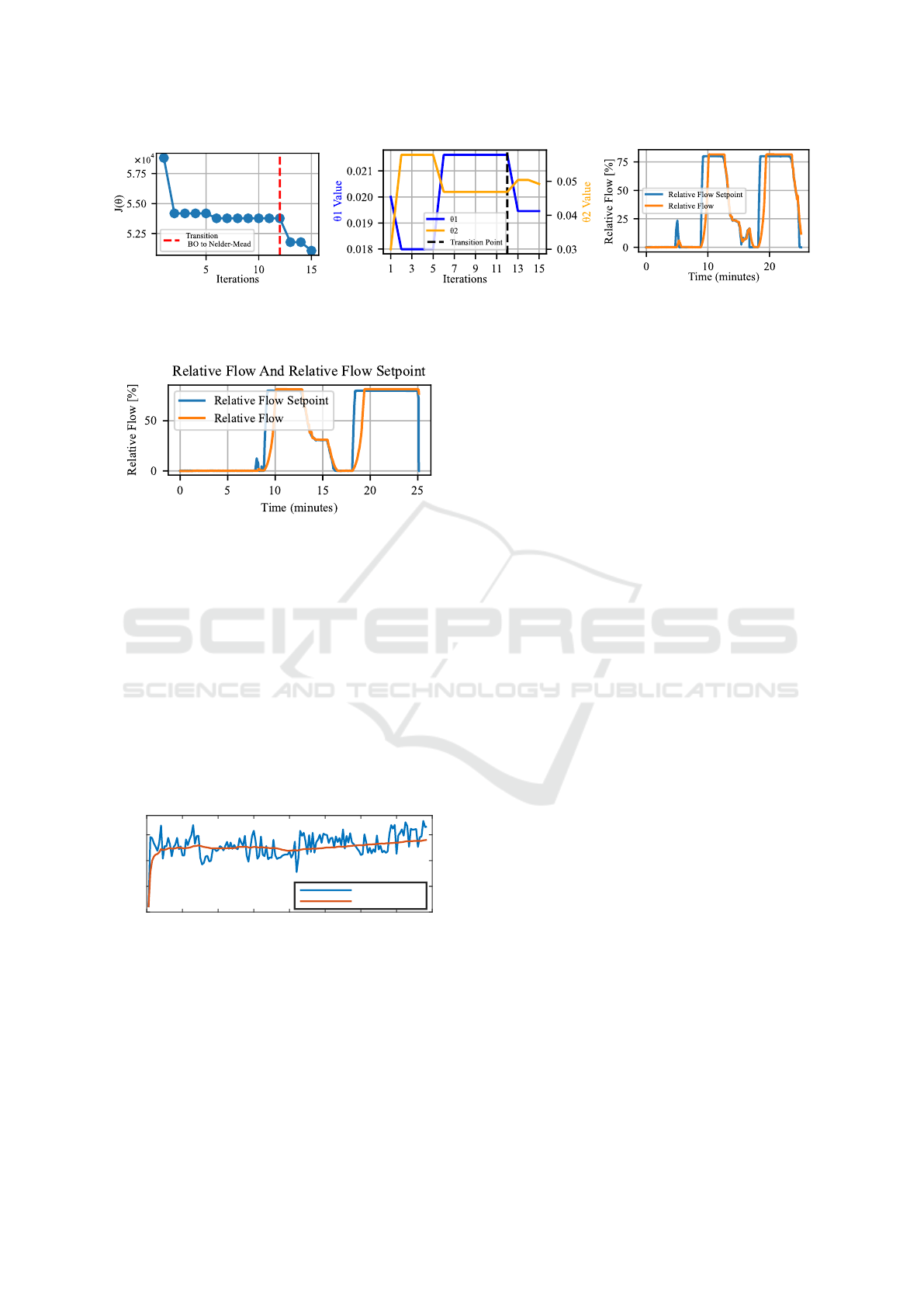
This section introduces the results obtained during

ofﬂine optimization with empirically derived heuristic

proﬁles as shown in Figure 1 (part 1).

As an initial step in our optimization process we

had to identify the optimal weights for Equation (1).

To balance the contribution of each design objective in

this cost function, we deﬁned an additional objective

function that scales each component by its correspond-

ing weight and aims to minimize the variance among

the scaled components. See the Appendix for detailed

results. We used these aligned weights to guide both

the initial and subsequent optimization phases. By

minimizing the variance of the scaled components, we

made sure that no design objective dominated and en-

sured that the optimization process can explore the

parameter space. This optimization progress is shown

in Figure 4a.

Figure 4b illustrates further modiﬁcation of the

parameters due to Nelder-Mead. Although this devel-

opment does not have a strong impact on our objective

function, it shows that our algorithm is searching to-

wards potential better values to further minimize our

non-penalized terms of objective function.

The optimized controller’s performance on the

heuristic stepwise setpoint proﬁle, as illustrated in Fig-

ure 4c demonstrates stable setpoint tracking with low

response times and no oscillations.

SIMULTECH 2024 - 14th International Conference on Simulation and Modeling Methodologies, Technologies and Applications

436

(a) (b) (c)

Figure 4: Experimental results, heuristic setpoint proﬁle. (a) Progress of objective function during optimization. (b) Progress of

tuning parameters. (c) Controller performance after optimization on a heuristic setpoint proﬁle.

4.2 Automated Tuning with Clustered

Setpoint Proﬁles

In this section we present our results from applying

black-box optimization on clustered setpoint proﬁle

as discussed in Section 3.2. The ﬁrst step involves

clustering of typical setpoint proﬁles collected over a

year. We use a single fully connected layer for both

the encoder and decoder neural networks. We refer

the reader to the appendix for a description of the au-

toencoder and its training setup. Here the combination

of 4000 epochs and a dimensionality of 4 yielded the

best results (see Figure 11a and Figure 11b). We cal-

culate the optimal number of clusters by applying grid

search using the silhouette score. Figure 5a shows the

improvement in the cost function with optimization

steps.

In Figure 5b the progress of the controller parame-

ters is illustrated. Especially noticeable is the further

optimization towards a minimum during the Nelder-

Mead phase. After the ﬁnal optimization of the param-

eters, the performance of the controller on a clustered

setpoint proﬁle is shown in Figure 5c.

Furthermore, to examine how well these parame-

ters generalize, we test them on our clustered setpoint

signal generated for the testing phase. The ﬂow track-

ing results shown in Figure 6 demonstrate satisfactory

tracking performance.

4.3 Reinforcement Learning

This section presents the results attained by applying

SAC, by directly connecting it to the hydraulic circuit

simulation in closed-loop feedback. We do not assume

any form of pre-training on the actor model since our

objective is to demonstrate that a suitably exploring

RL policy such as SAC can learn to control the ﬂow

setpoint in an online setting. Therefore, our conﬁgura-

tion corresponds to the scratch conﬁguration of online

RL as described in (Zhang et al., 2023).

The objective function from Equation (5) was im-

plemented using standard blocks and functions in

Simulink. For implementing RL, we used the Rein-

forcement Learning Toolbox

from MATLAB

(The

MathWorks Inc., 2024). Due to the toolbox being

speciﬁcally suited for episodic RL instead of online

RL, we carried out the experiments in the episodic

setting. However, note that demonstrating success-

ful learning and control performance through episodic

learning is equivalent to proving it in the online setting.

This is because the algorithm employed is an off-policy

RL strategy that updates the policy network at every

step of the environment episode by uniformly sam-

pling a minibatch of data from a circular experience

buffer. In fact, if we just assume that the initial condi-

tion of every new episode is the exact same as where

the previous episode ended, then the chain of episodes

is indistinguishable from online learning. It is because

of this reason that time weighing is not considered for

the oscillation error term, otherwise, this equivalence

to online RL will no longer hold. One important dis-

tinction between episodic and online learning is that

when the episodes start with a random initial condition

the samples from episodic learning cover a large por-

tion of the distribution since random explorations in

online learning can only be in the neighborhood of the

current state. Thus episodic learning in this sense may

lead to faster convergence to the optima.

The RL agent is integrated with the system such

that its actions are added to the base PI ﬂow con-

troller’s signal according to Equation (4). This addition

allows the base PI controller to act like a pre-stabilizer

to the system when the initially untrained SAC policy

behaves like white noise making sure that the system

doesn’t exhibit dangerous behavior. Note that the base

PI controller parameters are obtained from the ofﬂine

optimization step, and for this experiment, we used

heuristic setpoint proﬁles.

The set of observations to the RL agent comprised

of the current error, the current setpoint, and the cur-

rent control input calculated by the base PI controller.

To allow the agent to learn to predict the system dy-

namics, and to make sure it receives the full set of

Integrated Data-Driven Framework for Automatic Controller Tuning with Setpoint Stabilization Through Reinforcement Learning

437

(a) (b) (c)

Figure 5: Experimental results, clustered setpoint proﬁle. (a) Progress of objective function during optimization. (b) Progress

of tuning parameters. (c) Controller performance after optimization on a clustered proﬁle from the training set.

Figure 6: Controller performance after optimization on a

clustered proﬁle from the test set.

information due to the non-markovianity induced by

non-linearities like deadzones and stiction, we also

feed the last 4 observations as input to the actor and

the critic networks. The base PI controller’s output

is given as an input in order to allow the RL agent

to learn its trends and make adjustments to yield an

overall optimal signal. Finally, note that the mean of

the actor distribution is allowed to be in the range of

[−1, 1]

to allow it to completely modify the PI ﬂow

controller’s control signal which lies in the range of

[0, 1]

. A saturation function is applied to the ﬁnal con-

trol signal from Equation (4) to restrict it in the valid

range of [0, 1].

0 20 40 60 80 100 120 140 160

Episode Number

-800

-600

-400

-200

Episode Reward

Episode Rewards

Average Rewards

Figure 7: Episode reward trend along with the average return.

Figure 7 shows the trend of the variation in total

cost throughout the episode. It can be observed that

the algorithm improves rapidly in the initial episodes

and then seems to plateau when it cannot learn further

based on the information provided. Being an entropy

maximizing algorithm one observes consistent gradual

improvement even after 160 episodes (approx. 2.8M

samples).

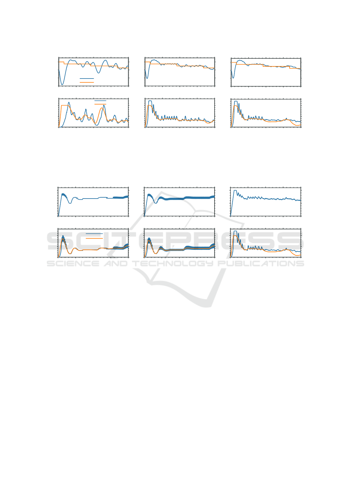
Figure 8 shows the comparison between the closed

loop control response of the trained and untrained SAC

agents, demonstrating the improvement in setpoint

tracking performance as training progresses. A com-

parison between the setpoint tracking performance of

the ofﬂine optimized PI ﬂow controllers and the con-

troller with the online optimized RL agent added to

it is shown in Figure 9. The error signal fed to the

RL and the PI controller encounters a deadzone near

the zero-point. This non-linearity leads to the error

being zero near the setpoint which is why the RL agent

doesn’t get penalized for small oscillations. The di-

rection change and oscillation terms make up for this

shortcoming and lead to gradual improvement in re-

moving oscillatory behavior by the agent. See the

Appendix for the SAC hyperparameters conﬁguration

and the actor-critic network architectures used in the

experiments.

5 CONCLUSION

In this paper, we presented a data-driven model-free

framework for automatic controller tuning and online

adaptation with setpoint stabilization in coupled sys-

tems. We experimentally demonstrated that our ap-

proach works on realistic scenarios in unknown sys-

tems with undetermined coupling relationships and

is, therefore, applicable to a broad range of practical

systems. We also showed that the last step of further

optimizing the controller online to its speciﬁc environ-

ment is crucial to obtain a better performing controller.

Our example of a cascaded control system is om-

nipresent in HVAC systems, and is applicable to a

large variety of systems encountered in control sys-

tems design. It is well known that such systems of

cascaded controller conﬁgurations quickly become un-

stable and traditional solutions which rely on adjusting

their time-constants to differ by an order of magnitude

are not optimal. We believe that the notion of learn-

ing to stabilize the control setpoint and minimize a

cost function with online learning is a key ingredient

SIMULTECH 2024 - 14th International Conference on Simulation and Modeling Methodologies, Technologies and Applications

438

0 450 900 1350 1800

Temperature (°C)

Temperature

Temperature Setpoint

0 450 900 1350 1800

Time (seconds)

0.5

Relative Flow

Water Flow

Flow Setpoint

(a) Agent after episode 2.

0 450 900 1350 1800

Temperature (°C)

0 450 900 1350 1800

Time (seconds)

0.5

Relative Flow

(b) Agent after episode 137.

0 450 900 1350 1800

Temperature (°C)

0 450 900 1350 1800

Time (seconds)

0.5

Relative Flow

Figure 8: Setpoint tracking performance comparison of the RL agent at different phases in the training. The labels mention the

number of episodes the agent has been trained for. Observe how the agent ﬁrst learns to minimize the error and eventually

reduces the number of actuator oscillations. Each plot shows the supply air temperature tracking the temperature setpoint (top)

and the ﬂow setpoint with the actual water ﬂow (bottom). In all cases the trained trained policy is still sampling actions from

the random distribution.

0 450 900 1350 1800

0.5

Controller Output

0 450 900 1350 1800

Time (seconds)

0.5

Relative Flow

Water Flow

Flow Setpoint

(a) Heuristic setpoint proﬁles trained PI.

0 450 900 1350 1800

0.5

Controller Output

0 450 900 1350 1800

Time (seconds)

0.5

Relative Flow

(b) Clustered setpoint proﬁle trained PI.

0 450 900 1350 1800

0.5

Controller Output

0 450 900 1350 1800

Time (seconds)

0.5

Relative Flow

Figure 9: Setpoint tracking performance comparison of the controllers obtained after the 3 different stages. The RL agent

is operating on top of the clustered proﬁle trained PI ﬂow controller. Note that the currently used setpoint proﬁle is quite

different from the ones considered for the PI base controller in stages 1 and 2. The training proﬁles were changing stepwise for

which the PI controllers learned to converge as fast as possible without oscillations due to Equation (1). Thus, they are too

sharply tuned for the smooth and continuous ﬂow stepoint they receive from the temperature controller which leads to the

oscillations observed in (a) and (b). The RL agent adapts to this new unseen proﬁle and, therefore, performs better than the

ofﬂine optimized parameters after being trained online as can be seen in (c) which validates the requirement for online learning.

towards optimal control and adaptation in an online

setting. We do not claim that our combination of al-

gorithms for each step of the framework is the best,

since there are several more combinations of ofﬂine

and online policies learned through other strategies

which may be better. However, this work is an impor-

tant step towards achieving optimal online adaptive

control and presents a new paradigm for data-driven

controller design.

5.1 Future Work

For this work, we applied our optimization on a sim-

ulated hydraulic circuit without any variations. To

achieve a more generalized ﬁnal solution, we plan

to introduce variations into our plant and expand our

scope by exploring other application types, such as air

or refrigeration applications.

This work trained an RL agent from scratch by

applying it directly to the system in a closed loop set-

ting. It is worth exploring other strategies such as

actor-critic pre-training on base controller data before

gradually deploying the RL Policy as done in (Soli-

nas et al., 2024). Furthermore, several strategies like

imitation learning on ofﬂine data, policy expansion of

ofﬂine trained policies by bridging them with online

trained policies, etc. are worth exploring as discussed

in (Zhang et al., 2023).

Integrated Data-Driven Framework for Automatic Controller Tuning with Setpoint Stabilization Through Reinforcement Learning

439

The problem of instability in cascaded controllers

also extends to the setting of networked control sys-

tems. To take an example from the setting presented in

this paper, oftentimes several temperature control units

send ﬂow setpoints to multiple ﬂow control valves

which are connected to the same hydraulic circuit and

thus have unknown physical coupling effects between

each other thus rendering any single-agent control law

suboptimal and potentially destabilizing. It may thus

be interesting to learn the physical dependencies of the

cascaded controllers and leverage this information to

stabilize such controller networks. This directly leads

the research in the direction of multi-agent reinforce-

ment learning. We propose to continue research on

these ideas and extend the framework we present in

this work accordingly.

ACKNOWLEDGEMENTS

We are indebted to Volkher Scholz for his many in-

valuable ideas and insights which helped shape the

contents of this paper and for proofreading several

drafts of this paper. We further extend our gratitude

to Stefan Mischler for his support and helpful advice,

enabling us to achieve the presented results. Also we

would be remiss not to thank the team at MathWorks

who helped us out with many helpful clariﬁcations and

support. Last but not least, we would like to thank

our colleagues for many stimulating and motivating

discussions.

REFERENCES

Ahmad, M. A., Ishak, H., Nasir, A. N. K., and Ghani, N. A.

(2021). Data-based pid control of ﬂexible joint robot us-

ing adaptive safe experimentation dynamics algorithm.

Bulletin of Electrical Engineering and Informatics.

Cohen, G. H. and Coon, G. A. (2022). Theoretical Considera-

tion of Retarded Control. Transactions of the American

Society of Mechanical Engineers, 75(5):827–834.

Esraﬁlian-Najafabadi, M. and Haghighat, F. (2023). Trans-

fer learning for occupancy-based HVAC control: A

data-driven approach using unsupervised learning of

occupancy proﬁles and deep reinforcement learning.

Energy and Buildings, 300:113637.

Fiducioso, M., Curi, S., Schumacher, B., Gwerder, M., and

Krause, A. (2019). Safe contextual bayesian optimiza-

tion for sustainable room temperature pid control tun-

ing. In Proceedings of the Twenty-Eighth International

Joint Conference on Artiﬁcial Intelligence, IJCAI-19,

pages 5850–5856. International Joint Conferences on

Artiﬁcial Intelligence Organization.

Fux, S. F., Mohajer, B., and Mischler, S. (2023). A compari-

son of the dynamic temperature responses of two differ-

ent heat exchanger modelling approaches in simulink

simscape for HVAC applications. In Wagner, G.,

Werner, F., and Rango, F. D., editors, Proceedings

of the 13th International Conference on Simulation

and Modeling Methodologies, Technologies and Appli-

cations, SIMULTECH 2023, Rome, Italy, July 12-14,

2023, pages 417–424. SCITEPRESS.

Gaing, Z.-L. (2004). A particle swarm optimization approach

for optimum design of pid controller in avr system.

IEEE Transactions on Energy Conversion, 19(2):384–

391.

Gao, F. and Han, L. (2012). Implementing the Nelder-Mead

simplex algorithm with adaptive parameters. Computa-

tional Optimization and Applications, 51(1):259–277.

Garcia, C. E. and Morari, M. (1982). Internal model control.

a unifying review and some new results. Industrial &

Engineering Chemistry Process Design and Develop-

ment, 21(2):308–323.

Goodfellow, I., Bengio, Y., and Courville, A. (2016). Deep

Learning. MIT Press.

Haarnoja, T., Zhou, A., Abbeel, P., and Levine, S. (2018).

Soft Actor-Critic: Off-Policy Maximum Entropy Deep

Reinforcement Learning with a Stochastic Actor. Tech-

nical report. arXiv:1801.01290 [cs, stat] type: article.

Haarnoja, T., Zhou, A., Hartikainen, K., Tucker, G., Ha,

S., Tan, J., Kumar, V., Zhu, H., Gupta, A., Abbeel, P.,

and Levine, S. (2019). Soft actor-critic algorithms and

applications. (arXiv:1812.05905). arXiv:1812.05905

[cs, stat].

Hazan, E., Lee, H., Singh, K., Zhang, C., and Zhang, Y.

(2018). Spectral Filtering for General Linear Dynami-

cal Systems. In Proceedings of the 32nd International

Conference on Neural Information Processing Systems,

NIPS’18, pages 4639–4648, Red Hook, NY, USA. Cur-

ran Associates Inc.

Kingma, D. P. and Ba, J. (2017). Adam: A method for

stochastic optimization.

MacQueen, J. (1965). Some methods for classiﬁcation and

analysis of multivariate observations. Proceedings of

the Fifth Berkeley Symposium on Mathematical Statis-

tics and Probability (June 21-July 18, 1965 and Decem-

ber 27, 1965-January 7, 1966), pages pages 281–297.

Referenced by: MathSciNet [MR0214227].

Mnih, V., Kavukcuoglu, K., Silver, D., Graves, A.,

Antonoglou, I., Wierstra, D., and Riedmiller, M. A.

(2013). Playing atari with deep reinforcement learning.

CoRR, abs/1312.5602.

Mok, R. and Ahmad, M. A. (2022). Fast and optimal tuning

of fractional order pid controller for avr system based

on memorizable-smoothed functional algorithm. En-

gineering Science and Technology, an International

Journal.

Neumann-Brosig, M., Marco, A., Schwarzmann, D., and

Trimpe, S. (2020). Data-efﬁcient autotuning with

bayesian optimization: An industrial control study.

IEEE Transactions on Control Systems Technology,

28(3):730–740.

Rasmussen, C. E. and Williams, C. K. I. (2005). Gaussian

Processes for Machine Learning. The MIT Press.

SIMULTECH 2024 - 14th International Conference on Simulation and Modeling Methodologies, Technologies and Applications

440

Recht, B. (2018). A tour of reinforcement learning: The

view from continuous control. (arXiv:1806.09460).

arXiv:1806.09460 [cs, math, stat].

Solinas, F. M., Macii, A., Patti, E., and Bottaccioli, L.

(2024). An online reinforcement learning approach

for HVAC control. Expert Systems with Applications,

238:121749.

Stenger, D. and Abel, D. (2022). Benchmark of bayesian op-

timization and metaheuristics for control engineering

tuning problems with crash constraints.

Sutton, R. S. and Barto, A. G. (2020). Reinforcement Learn-

ing: An Introduction. Adaptive Computation and Ma-

chine Learning Series. The MIT Press, second edition

edition.

The MathWorks Inc. (2024). Matlab version: 23.2.0

(r2023b).

Yu, Z., Yang, X., Gao, F., Huang, J., Tu, R., and Cui, J.

(2020). A Knowledge-based reinforcement learning

control approach using deep Q network for cooling

tower in HVAC systems. In 2020 Chinese Automation

Congress (CAC), pages 1721–1726.

Zhang, H., Xu, W., and Yu, H. (2023). Policy expansion

for bridging ofﬂine-to-online reinforcement learning.

(arXiv:2302.00935). arXiv:2302.00935 [cs].

Zhang, X., Xie, Y., Han, J., and Wang, Y. (2022). Design of

control valve with low energy consumption based on

isight platform. Energy, 239:122328.

Zhuang, D., Gan, V. J. L., Duygu Tekler, Z., Chong, A., Tian,

S., and Shi, X. (2023). Data-driven predictive control

for smart HVAC system in IoT-integrated buildings

with time-series forecasting and reinforcement learn-

ing. 2023, 338:120936.

Ziegler, J. G. and Nichols, N. B. (1993). Optimum Settings

for Automatic Controllers. Journal of Dynamic Sys-

tems, Measurement, and Control, 115(2B):220–222.

Astr

om, K. and H

agglund, T. (2004). Revisiting the

ziegler–nichols step response method for pid control.

Journal of Process Control, 14(6):635–650.

APPENDIX

SAC Hyperparameters

Table 1 lists the hyperparameter conﬁguration used

for training the Soft-Actor critic agent mentioned in

Section 4.3.

Actor-Critic Networks

Figure 10 shows the neural-network architectures used

for the actor and the critic networks. The observation

input to the critic network (Figure 10a) is 15 dimen-

sional since the set of observations at a given time-step

consists of 3 scalars, and we feed the last 4 obser-

vations along with the current time-step to both the

networks. In the actor net (Figure 10b) tanh layer is

used to allow the mean action to be in

[−1, 1]

to allow

full range modiﬁcation of the base PI ﬂow controller’s

signal, while a softplus layer is used to ensure pos-

itive values for the standard deviation of the action

distribution.

Action Observation

QValue

Concat

Dense

ReLU

Dense

ReLU

Dense

1 15

(a) Critic Network.

Observation

stddev_action

mean_action

Dense

ReLU

Dense

Softplus

15 15

Dense

Tanh

(b) Actor Network.

Figure 10: SAC actor and critic neural network architectures.

Bayesian Optimization, Clustering and

Autoencoder Training

The optimized weights for different setpoint proﬁles

are shown in Table 2.

Autoencoder Networks

The autoencoder consists of an encoder network and

a decoder network. For both networks we choose

simple one layer neural networks. The encoder has the

Table 1: SAC hyperparameter conﬁguration.

Parameter Value

Optimizer

Adam (Kingma and

Ba, 2017)

Learning rate 0.001

Discount factor (γ) 0.99

Minibatch size 256

Entropy target −1(−dim(A))

Target smoothing coeff. (

)

0.001

Target update frequency 1

Policy update frequency 1

Gradient steps 1

Replay buffer size 10

Number of warm start steps

1810

Episode length 1800

Number of episodes 126

Simulation time step 0.1 sec

(λ

, λ

) 10

−2

·(6, 1.6, 1, 0.1)

Integrated Data-Driven Framework for Automatic Controller Tuning with Setpoint Stabilization Through Reinforcement Learning

441

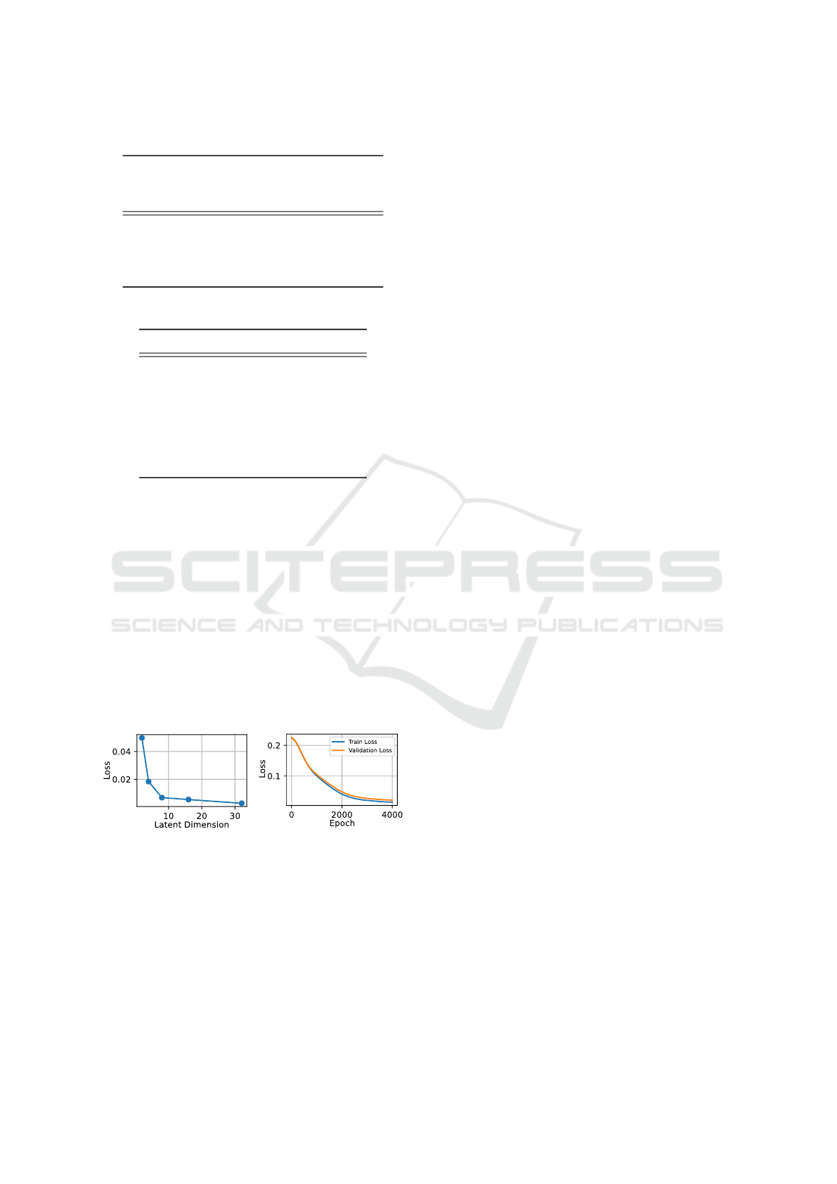
Table 2: Optimized weights for different setpoint proﬁles.

Weight

Heuristic Set-

point Proﬁle

Clustered

Setpoint

Proﬁle

Weight 1 1.11777344 1.20485840

Weight 2 2.24179687 2.09331055

Weight 3 704.68750 1082.29980

Weight 4 3036.91406 2000.00000

Table 3: Autoencoder training hyperparameters.

Parameter Value

Optimizer Adam

Learning Rate 10

−4

0.9

0.999

Batch size 64

Epochs 3000

Loss Function Mean Squared Error

following structure

1. Fully Connected Layer (1000 → 4)

2. ReLU

And the decoder has a similar architecture

1. Fully Connected Layer (4 → 1000)

2. Sigmoid

The hyperparameters used for training are listed in

Table 3.

Clustering

See Figure 11a and Figure 11b.

(a) (b)

Figure 11: (a) Validation losses of last epoch for different

latent dimensions. (b) Training and validation losses over

epochs.

SIMULTECH 2024 - 14th International Conference on Simulation and Modeling Methodologies, Technologies and Applications

442