Research on the Control of the end Effector of the Large-Scale

Curved Surface Compliant Polishing Robot

Runyang Zhan

Ningbo Institute of Technology, Zhejiang University, Ningbo, 315000, China

Keywords: Path Planning, Particle Swarm Optimization, Tuna Swarm Optimization.

Abstract: Curved surface parts find extensive use in various applications, and their surface quality plays a crucial role

in their performance. Industrial robot technology has advanced to the point where manual polishing can be

replaced. However, most robots currently employ position control, which has low accuracy in force control

and is unsuitable for the task. This paper aims to address the limitations of current research by focusing on an

improved control strategy that uses a parameter optimization algorithm to enhance the system's dynamic

performance. The main areas of research include the control of the end effector's contact force. Firstly, a

mathematical model of the pneumatic control loop is established and the system transfer function is obtained

through system identification. An improved optimization algorithm based on Particle Swarm Optimization

and Tuna Swarm Optimization is proposed to enhance the mechanism's control performance when dealing

with complex nonlinear systems. This algorithm has a faster convergence speed, higher convergence accuracy,

and stronger searchability.

1 INTRODUCTION

There has been some progress in the research of flat

automatic polishing due to the advancements in

industrial robot application technology. However,

there are still some problems to be solved in the

application of robots in the field of large curved

surface compliance polishing.

Managing compliance force for large curved

surfaces presents a challenging task due to strong

coupling, nonlinearities, and frequent changes. The

traditional control method's utilization is insufficient

to allow for the real-time adaptive adjustment of the

control proportional coefficient. This leads to

inadequate system performance and the incapability

to maintain a stable and consistent force processing

target. To enhance the control effect, it is imperative

to implement a control strategy that is combined with

a parameter optimization algorithm.

In the 21st century, robot technology has emerged

as a major high-tech industry that is playing a crucial

role in the lives and work of people across the globe.

With rapid developments in other industries like

automobiles and computers, robots are now widely

used in electrical and electronics, automobile, metal

and machinery manufacturing, plastics and chemistry,

food and beverage, and other industries. Industrial

robots are highly regarded in academia and industry

because of their flexibility, excellent motion stability,

and high-precision repetitive trajectory motion in a

large workspace (Yu 2020). Despite COVID-19's

impact on the industry in the first two years, the total

number of industrial robots installed worldwide has

continued to increase, with a ten-year growth rate of

211%. It is predicted that the number of industrial

robots installed globally will exceed 690,000 by 2025.

In today's technological era, using robots for

grinding and polishing is more popular than

traditional manual methods. This is especially useful

for large, curved parts that have complex and uneven

surface profiles, requiring precision in both profile

and surface finish. Nonetheless, it is worth noting that

industrial robots have lower position accuracy and

repeatability accuracy when compared to Computer

Numerical Control (CNC) machine tools (Zhang

2021). When it is located in different spatial poses, its

stiffness difference (Wen & Pagilla 2021) and

dynamic characteristic change (Amersdorfer et al.

2020) are relatively large, which will lead to

unpredictable processing vibration and structural

deformation (Zhu et al. 2022) during the polishing

process, and cannot achieve the expected processing

target. Therefore, it is necessary to It is considered to

Zhan, R.

Research on the Control of the end Effector of the Large-Scale Curved Surface Compliant Polishing Robot.

DOI: 10.5220/0012869900004547

Paper published under CC license (CC BY-NC-ND 4.0)

In Proceedings of the 1st International Conference on Data Science and Engineering (ICDSE 2024), pages 599-607

ISBN: 978-989-758-690-3

599

adjust and optimize the sensor technology to monitor

the grinding and polishing process by designing and

improving the control algorithm.

In recent years, there has been substantial research

conducted on the technology of curved surface

polishing utilizing robots, both domestically and

internationally. Many scholars have analyzed the

limitations inherent in the existing tool contact state

research and have proposed new and improved

methods. For instance, Xie Liujie of South China

University of Technology has enhanced the surface

material removal depth model, proposing a multi-

directional three-dimensional curved surface grinding

and polishing optimization cycloidal machining

trajectory based on the Angle Based Flattening++

(ABF++) algorithm. This method was verified

through experimentation to improve process control

(Xie 2018). Furthermore, Zhang Sui of Soochow

University has focused on refining the polishing path

and process plan and processing Off-axis aspheric

mirror elements with good form error (Zhang 2021).

Yalun Wen et al. presented a new 3D path

tracking control framework based on the Hermite-

Simpson collocation method, which determines the

dynamically feasible Cartesian space processing path

and the maximum constant translation speed. They

built a robot for the 3D path tracking control grinding

and polishing experimental platform, which

improved the overall performance of the robot

grinding and polishing system and met the surface

finishing requirements of curved surface parts (Wen

& Pagilla 2021). Finally, Manuel Amersdorfer et al.

have proposed a method utilizing distance sensor data

to create an approximate model of surface

topography, replacing the traditional prior model.

They have built a free-form surface force-controlled

robot automatic polishing system for real-time path

tracking, which accurately controls the normal

contact force of grinding and polishing (Amersdorfer

et al. 2020).

To solve the problems in the above analysis, this

paper conducts the following innovative research.

Introducing a new parameter optimization algorithm

called Improved Tuna Swarm Optimization - Particle

Swarm Optimization (ITSO-PSO) combines tuna

with particle swarm optimization. This algorithm

boasts fast convergence speeds, high precision, and

excellent search capabilities. It excels at dynamic

tuning of control parameters and performs well on

complex nonlinear multivariable systems with

minimal overall error.

2 PARAMETER OPTIMIZATION

2.1 Particle Swarm Optimization

Algorithm

The Particle Swarm Optimization (PSO) algorithm is

a type of swarm intelligence evolutionary algorithm

utilized to optimize nonlinear functions. Its creation

is credited to James Kennedy, an American

psychologist, and Russell Eberhart, an electrical

engineer, in 1995 (Kennedy & Eberhart 1995).

Taking inspiration from the foraging behavior of

birds, the algorithm treats a flock of birds as massless

particles. The positions the particles pass through

during flight are considered potential solutions to the

optimization problem at hand. As particles fly, they

search for viable solutions, their velocity and position

being the key factors influencing their progress.

Further, extend the particle to n-dimensional space,

then the position vector 𝑋





𝑥



,𝑥



,⋯,𝑥





particle i in n-dimensional space, and the flight

velocity vector 𝑉





𝑣



,𝑣



,⋯,𝑣





. Choose the

suitable fitness calculation function as the test

function, assign the initial position and speed to the

particle swarm randomly, identify the optimal

position of an individual particle and the group of

particles at present, evaluate the fitness of the particle,

and progressively revise the position and velocity of

the swarm until the ultimate position of the particle

swarm is attained.

The speed iteration of the classic PSO algorithm

is shown in equation (1), and the position iteration is

shown in equation (2),

(𝑉_𝑖^(𝑘 + 1)=𝑤𝑉_𝑖^𝑘+ 𝑐_1 𝑟_1 (𝑃_𝑏𝑒𝑠𝑡 − 𝑋_𝑖^𝑘 ) +

𝑐_2 𝑟_2 (𝐺_𝑏𝑒𝑠𝑡− 𝑋_𝑖^𝑘 ),)

(1)

𝑋





=𝑋





+𝑉





. (2)

The equation includes several variables: k

denotes the current iteration number of the particle,

while w represents the inertia factor, which balances

global and local optimization. Additionally, 𝑐



and 𝑐



represent learning factors, which reflect individual

and group cognitive abilities respectively, and 𝑟



and

𝑟



represent random numbers within the range [0,1].

Finally, uppercase 𝑃



represents the optimal

position of a single particle, while uppercase 𝐺



represents the optimal position of the entire particle

group.

To initiate the PSO algorithm process, the first

step entails initializing the particle swarm. This

includes randomly generating the starting position

and velocity, as well as selecting appropriate values

for the number of iterations, population size, particle

dimension, inertia factor, and learning factor. In the

subsequent step, a fitness function is adopted and

ICDSE 2024 - International Conference on Data Science and Engineering

600

employed to compute the fitness value of each

particle. The third step involves updating each

particle by comparing its fitness with its historical

optimal value. The fourth step involves updating the

particle swarm by comparing each particle's fitness

with its historical optimal value. In the fifth step, the

velocity and position of the particles are updated

according to equations (1) and (2). Finally, the loop

end condition is evaluated to determine if it has been

met. If not, the process returns to step 2 and continues

to execute.

2.2 Tuna Swarm Optimization

Algorithm

The Tuna Optimization Algorithm (TSO) is a global

meta-heuristic optimization algorithm that simulates

the spiral and parabolic foraging behaviors of tuna in

a swarm-based approach (Xie et al. 2021). Tuna

employs distinct foraging methods, namely the spiral

and parabolic techniques. The spiral approach

involves swimming in an upward spiral to contain

their prey in a confined area for more efficient

feeding, while the parabolic technique entails chasing

the tuna in front of them to create a parabolic shape

for capturing prey. As for initializing particles for the

TSO algorithm, a precise calculation equation is

implemented,

𝑌



=𝑟𝑎𝑛𝑑⋅

(

𝑏



−𝑏



)

+𝑏



(

)

where 𝑌



represents the initial position of the tuna,

and 𝑏



and 𝑏



represent the maximum and

minimum values of the search range. Further, the

position of the tuna population during spiral foraging

can be deduced,

𝑌





⎩

⎪

⎨

⎪

⎧

𝛼



⋅(𝑌





+𝛽⋅𝑌





−𝑌





) + 𝛼



⋅𝑌





,𝑘=1；𝑟𝑎𝑛𝑑<

𝑘

𝑚

𝛼



⋅𝑌





+𝛽⋅𝑌





−𝑌





 + 𝛼



⋅𝑌





,𝑘𝜖



2,𝑚



；𝑟𝑎𝑛𝑑<

𝑘

𝑚

𝛼



⋅𝑌





+𝛽⋅𝑌





−𝑌





 + 𝛼



⋅𝑌





,𝑘=1；𝑟𝑎𝑛𝑑≥

𝑘

𝑚

𝛼



⋅𝑌





+𝛽⋅𝑌





−𝑌





 + 𝛼



⋅𝑌





,𝑘𝜖



2,𝑚



；𝑟𝑎𝑛𝑑≥

𝑘

𝑚

(

)

The calculation equation of each coefficient is

𝛼



=𝛼



(

1−𝛼



)

∙

𝑘

𝑚

(

)

𝛼



(

1−𝛼



)

−

(

1−𝛼



)

⋅

𝑘

𝑚

(

)

𝛽=𝑒





⋅

⋅ cos

(

2𝜋𝛽



(

)

𝑙=𝑒



















(

)

where 𝑌





indicates the position of the jth particle

after the (𝑘+1)th iteration; 𝑌





indicates the

position of the current optimal particle; the subscripts

𝛼



and 𝛼



refer to weight coefficients that influence a

particle's movement towards the optimal particle and

its previous trend, respectively. These coefficients

effectively control the particle's ability to conduct

both global and local searches; 𝛼



indicates the

degree to which the particle follows the optimal

particle and the previous article in the initial state; k

indicates the current iteration number; m indicates the

maximum The number of iterations; 𝛽 represents the

coefficient of the particle and the optimal particle or

random particle, 𝛽



represents the random number in

the value range [0,1]; 𝑙 represents the coefficient

related to the maximum number of iterations m and

the current number of iterations k, there is no actual

physical meaning.

It is assumed that when feeding, tuna has a 50%

chance of choosing a parabolic path and a 50%

chance of feeding randomly. The mathematical model

𝑌





=

𝑌





+𝑟𝑎𝑛𝑑⋅(𝑌





−𝑌





)+𝑞⋅𝑝



⋅(𝑌





−𝑌





),𝑟𝑎𝑛𝑑<0.5

𝑞⋅𝑝



⋅𝑌





,𝑟𝑎𝑛𝑑≥0.5

(

)

𝑝=1−

𝑘

𝑚







(

)

where the value of q is {-1,1}, which determines the

direction of the particle swarm foraging; p reflects

the process of foraging.

Research on the Control of the end Effector of the Large-Scale Curved Surface Compliant Polishing Robot

601

2.3 Improved Optimization Algorithm

Based on Tuna and Particle Swarm

Optimization

When tackling intricate problems with numerous

dimensions, the conventional PSO algorithm may

present a few limitations. While it boasts a rapid

search space velocity, it lacks local search

capabilities, causing the optimization to potentially

settle into a local optimum. Furthermore, insufficient

information exchange between particles may lead to

sluggish convergence, hindering the attainment of the

optimal solution (Song et al. 2021). The ITSO-PSO

algorithm combines the advantages of both

algorithms to enhance global and local search

performance.

The speed and position iterative calculation

equations of the ITSO-PSO optimization algorithm

are

𝕍





⎩

⎨

⎧

𝑤𝕍





+𝑐



𝑟



𝑀



−𝑍





+𝑐



𝑟



𝑀



−𝑍





,𝑟𝑎𝑛𝑑<

𝑡

𝑚𝑎𝑥𝑔𝑒𝑛

𝑤𝕍





+𝑐



𝑟



𝑀



−𝑍





+𝑐



𝑟



𝐺



−𝑍





,𝑟𝑎𝑛𝑑≥

𝑡

𝑚𝑎𝑥𝑔𝑒𝑛

(

)

𝑍





⎩

⎨

⎧

𝑤⋅𝑍





+𝑤⋅𝕍





, 𝑟𝑎𝑛𝑑<

𝑡

𝑚𝑎𝑥𝑔𝑒𝑛

𝑤⋅𝑍





(

1−𝑤

)

⋅𝕍





,𝑟𝑎𝑛𝑑≥

𝑡

𝑚𝑎𝑥𝑔𝑒𝑛

(

)

𝑀



𝑃



+𝐺



(

)

where 𝕍





and 𝑍





represent the speed and

position of the gth particle after the (𝑡+1) iteration,

maxgen represents the maximum number of iterations,

and 𝑀



represents the particle's personal best best

position and group best position average.

The optimization capabilities of a particle swarm

are influenced by the inertia factor and the learning

factor. A larger inertia factor means weaker local

optimization capabilities, while a smaller one leads to

weaker global optimization. When the learning factor

𝑐



is small, particles may struggle with local search

and become stuck in suboptimal situations, unable to

reach the global optimal solution. Similarly, when 𝑐



is small, particles may not communicate enough,

slowing down convergence and preventing the

discovery of an optimal solution. Therefore, it is

necessary to properly improve and optimize the

inertia factor and learning factor (Zhao et al. 2014),

and the changes are

𝑤=0.5⋅

(

𝑤



+𝑤



)

+0.5⋅

(

𝑤



−𝑤



)

⋅𝑡𝑎𝑛ℎ−4+

8⋅

(

𝑚𝑎𝑥𝑔𝑒𝑛 − 𝑡

)

𝑚𝑎𝑥𝑔𝑒𝑛

,

(

)

𝑐



=𝑐+

(

𝑐



−𝑐

)

⋅

𝑡

𝑚𝑎𝑥𝑔𝑒𝑛

(

)

𝑐



(

𝑐−0.5

)

(

𝑐−𝑐



)

⋅

𝑡

𝑚𝑎𝑥𝑔𝑒𝑛

(

)

where 𝑤



and 𝑤



represent the initial value and final

value of the inertia factor respectively.

To begin the ITSO-PSO algorithm, several

parameters must be initialized, including the learning

factor, inertia weight, maximum evolution times,

population size, and fitness function dimension.

Additionally, the value range of speed and position

must be limited and a fitness function must be

selected. Following this, a population is randomly

generated and the speed and fitness of each particle

are calculated. The best fitness values of the

individual and the group are then calculated and

updated accordingly. The algorithm then iteratively

updates the inertia factor, learning factor, particle

swarm velocity, and position using a ala while

preventing them from exceeding their range. To avoid

getting stuck at a local optimum, mutation seeds are

added. The algorithm continues until the end

condition is met, at which point the descending

optimization curve is output.

2.4 ITSO-PSO Algorithm Performance

Test

To compare the effectiveness of the ITSO-PSO

algorithm with the PSO algorithm, we selected five

classic test functions and conducted comparative

testing to verify the performance change (Huang et al.

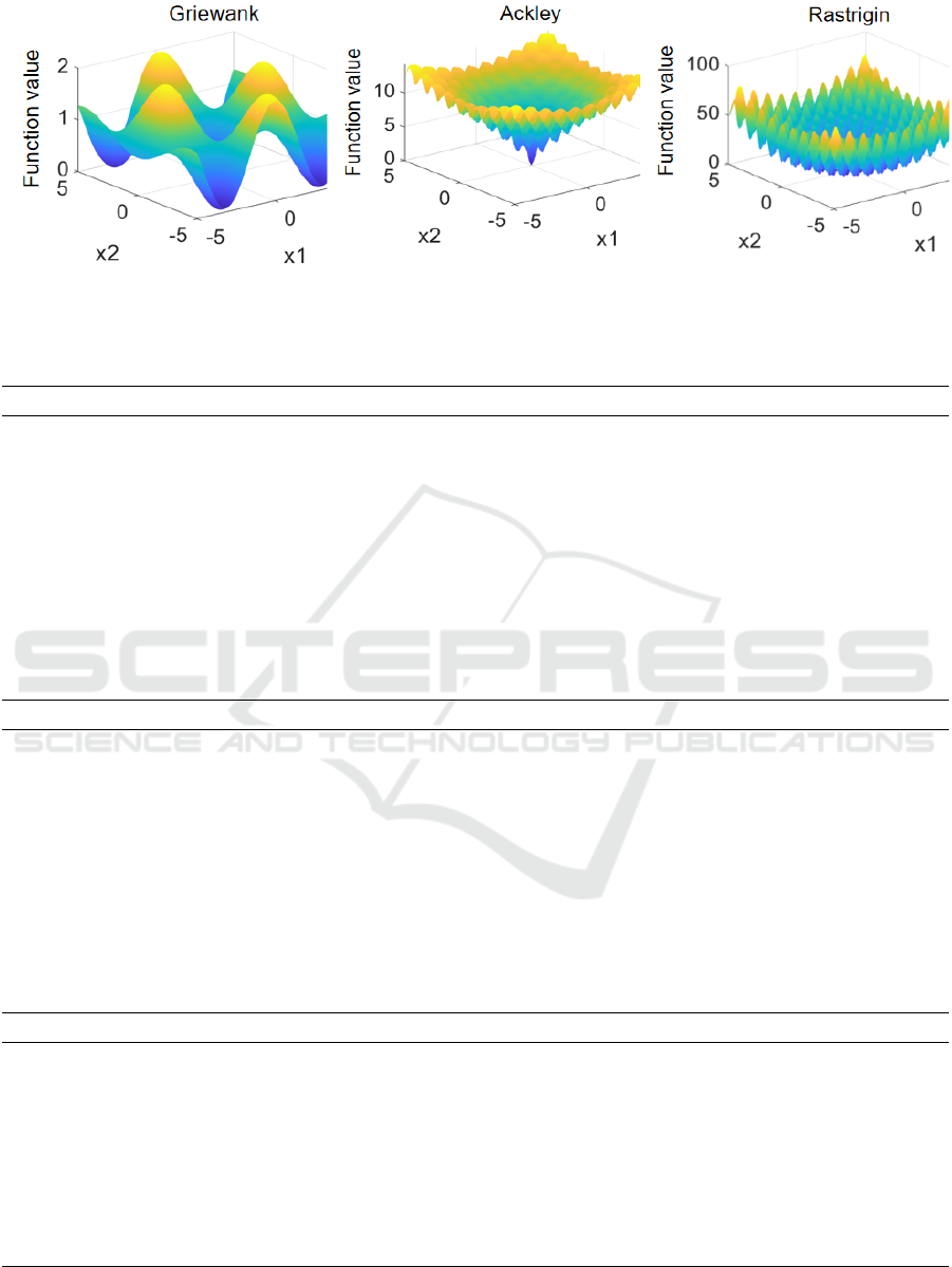
2018). In total, there are five test functions. Two of

them are unimodal test functions called Sphere and

Schwefel's Problem 2.22, which aid in determining

the algorithm's search accuracy and iteration rate. The

remaining three tests are multimodal test functions -

Griewank, Ackley, and Rastrigin - designed to

ICDSE 2024 - International Conference on Data Science and Engineering

602

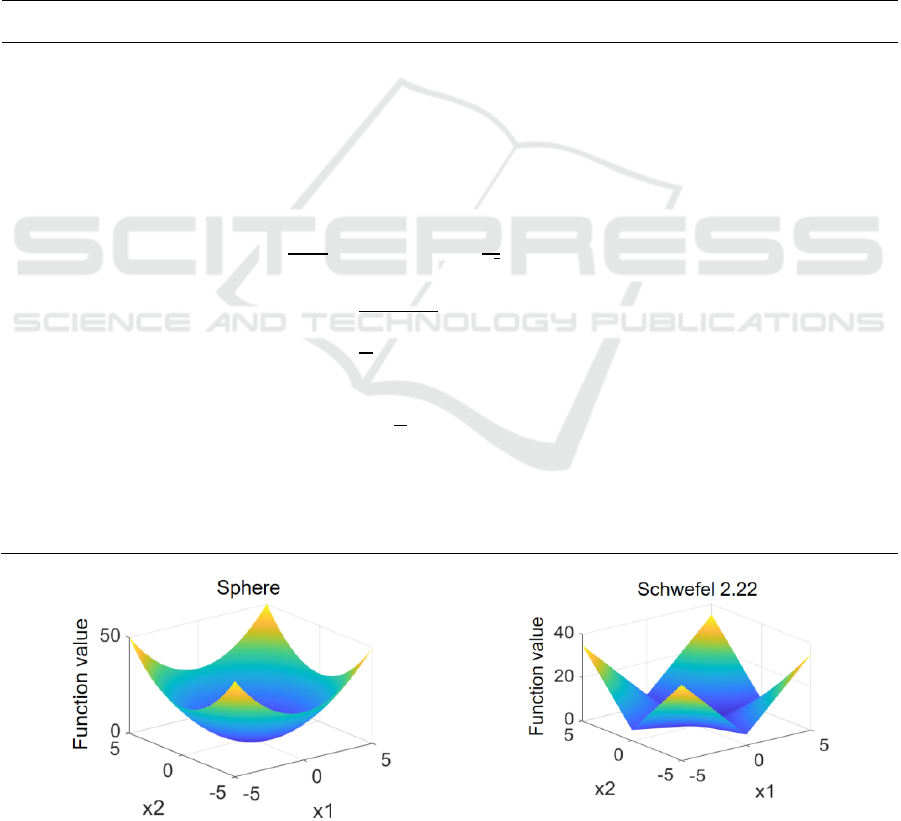
prevent the algorithm from converging prematurely

by avoiding local optima. Table 1 provides the

optimal values and value ranges for all five test

functions, while Figure 1 visually represents the

definition domain and value range of the test

functions in three dimensions.

Use MATLAB R2019b version for code writing

and simulation testing, set the maximum number of

population iterations 𝑚𝑎𝑥𝑔𝑒𝑛=200; population size

G=100; inertia weight correlation coefficient w=0.9,

𝑤



=0.9, 𝑤



=0.4; learning factor correlation

coefficient c=1.5, 𝑐



=1.49345, 𝑐



=1.44345; set the

speed value range [-1,1]; set the position range

according to Table 1. After defining the initial

parameters, a specific test function is selected, and

varying variable dimensions are independently tested

for both algorithms, with each test run 30 times. For

each test where the fitness function converges (i.e.

when the fitness value is less than 0.001), the average

(AVG), standard deviation (STD), maximum (MAX),

minimum (MIN), and mean (MEAN) number of

iterations are documented. In cases where the number

of iterations is 200 and the fitness value is greater than

or equal to 0.001, the function is classified as not

having converged, and MAX, MIN, and MEAN are

marked as DNE. The outcomes of each test are

meticulously analyzed and documented in Table 2,

Table 3, Table 4, Table 5, and Table 6.

Table 1: The basic situation of 5 classic test functions.

Name

Equation Range

Optimal

value

Sphere

𝑓



=

(

𝑥



)







[-100,100] 0

Schwefel 2.22

𝑓



=

𝑥







+

𝑥







[-10,10] 0

Griewank

𝑓



4000



(

𝑥



)







−cos

𝑥



√

𝑖







[-600,600] 0

Ackley

𝑓



=−20 ⋅ exp

⎝

⎛

0.2



𝑁



(

𝑥



)







⎠

⎞

−exp(

𝑁

cos(2𝜋𝑥



))+20+𝑒





[-32,32] 0

Rastrigin

𝑓



=𝑥





−10cos

(

2𝜋𝑥



)

+ 10





[-5.12,5.12] 0

(a) Sphere (

) Schwefel 2.22

Research on the Control of the end Effector of the Large-Scale Curved Surface Compliant Polishing Robot

603

(d) Ackle

(e)Rastrigin

ure 1: 3D visualization out

ut of test function.

Table 2: Comparison of 2 optimization algorithms for solving 5 test functions (variable dimension D=3).

Algorithm Index

𝑓



𝑓



𝑓



𝑓



𝑓



ITSO-PSO

AVG 0 0 0 0 0

STD 0 0 0 0 0

MAX 55 99 56 100 82

MIN 32 91 31 94 51

MEAN 46 95 44 98 66

PSO

AVG 0 0 0 0 0.13329

STD 0 0 0 0 0.33935

MAX 81 143 72 141 196

MIN 57 111 62 112 39

MEAN 73 128 67 130 110

Table 3: Comparison of 2 optimization algorithms for solving 5 test functions (variable dimension D=10).

Algorithm Index

𝑓



𝑓



𝑓



𝑓



𝑓



ITSO-PSO

AVG 0 0 0 0 0

STD

0 0 0 0 0

MAX 81 108 72 106 128

MIN 71 103 62 102 83

MEAN 76 106 68 104 89

PSO

AVG 0 0.00395 0 0.00093 5.98740

STD 0 0.00662 0 0.00007 3.40882

MAX 138 200 140 137 DNE

MIN 109 119 104 96 DNE

MEAN 126 169 119 114 DNE

Table 4: Comparison of 2 optimization algorithms for solving 5 test functions (variable dimension D=30).

Algorithm Index

𝑓



𝑓



𝑓



𝑓



𝑓



ITSO-PSO

AVG 0 0 0 0 0

STD

0 0 0 0 0

MAX 88 112 80 109 99

MIN 84 110 74 106 95

MEAN 86 111 77 108 96

PSO

AVG 0.00096 0.27348 0.00097 0.01208 23.64657

STD 0.00004 0.09489 0.00003 0.00351 9.75532

MAX 191 DNE 134 DNE DNE

MIN 138 DNE 91 DNE DNE

MEAN 168 DNE 115 DNE DNE

ICDSE 2024 - International Conference on Data Science and Engineering

604

Table 5: Comparison of 2 optimization algorithms for solving 5 test functions (variable dimension D=50).

Algorithm Index

𝑓



𝑓



𝑓



𝑓



𝑓



ITSO-PSO

AVG 0 0 0 0 0

STD

0 0 0 0 0

MAX 90 114 82 109 99

MIN 86 111 75 107 97

MEAN 88 112 78 108 98

PSO

AVG 0.00723 0.91041 0.00098 0.05423 40.34964

STD 0.00207 0.17174 0.00002 0.00980 14.06941

MAX DNE DNE 192 DNE DNE

MIN DNE DNE 154 DNE DNE

MEAN DNE DNE 169 DNE DNE

Table 6: Comparison of 2 optimization algorithms for solving 5 test functions (variable dimension D=100).

Algorithm Index

𝑓



𝑓



𝑓



𝑓



𝑓



ITSO-PSO

AVG 0 0 0 0 0

STD

0 0 0 0 0

MAX 92 115 82 109 100

MIN 87 113 77 106 98

MEAN 89 114 79 108 99

PSO

AVG 0.07823 2.64485 0.00169 0.14961 177.16030

STD 0.01089 0.22698 0.00023 0.01661 47.02125

MAX DNE DNE DNE DNE DNE

MIN DNE DNE DNE DNE DNE

MEAN DNE DNE DNE DNE DNE

Based on the simulation results outlined in the

table, it's clear that both algorithms can achieve

iterative test value convergence when the variable

dimension is low. However, the traditional PSO

algorithm requires more iterations, and as the

variable dimension increases, some of its test

functions fail to converge. If the variable dimension

reaches a critical point, the PSO algorithm won't

converge, and each evaluation performance

indicator parameter will decline to varying degrees.

By analyzing the change curves of the five test

degree functions shown in Figure 2, we can see that

the proposed ITSO-PSO optimization algorithm can

achieve the theoretical optimal solution in all test

scenarios, meaning that the test function can

converge in any scenario. Compared to the

traditional PSO algorithm, the ITSO-PSO algorithm

achieves convergence with fewer iterations,

indicating a faster convergence rate. Additionally,

the ITSO-PSO algorithm is more robust, even when

the variable dimension increases from 100 to 500.

The average number of convergence times when the

algorithm reaches convergence does not increase

significantly, making numerical variable space

parameter optimization a valuable reference point,

as shown in Figure 3.

(a) Sphere (

) Schwefel 2.22

Research on the Control of the end Effector of the Large-Scale Curved Surface Compliant Polishing Robot

605

(

)

Griewan

)

Ackle

(

)

Rastri

Figure 2: Five test function fitness change curves (D=100).

Figure 3: ITSO-PSO algorithm convergence times and variable dimension function curve.

In summary, the ITSO-PSO algorithm proposed

based on the TSO algorithm and the traditional PSO

algorithm solves the problem of premature

convergence that may fall into local extreme points

when solving complex nonlinear unimodal or

multimodal function problems. The test results show

that the ITSO-PSO algorithm has a fast convergence

speed, good global search ability and local search

ability, high convergence accuracy, and the ability to

optimize complex system parameters.

3 CONCLUSION

This paper centers around the precise manipulation of

the end effector on a polishing robot, specifically one

designed for curved surfaces. This paper has yielded

remarkable results thus far. This paper developed a

mathematical model that enables me to establish a

pneumatic control loop for each component and

pinpoint the transfer function of the pneumatic

control system. Ther proposed ITSO-PSO algorithm

has outperformed traditional PSO algorithms in terms

of faster convergence speed, increased accuracy, and

superior capabilities for both global and local

searches. Although the research has its limitations,

ICDSE 2024 - International Conference on Data Science and Engineering

606

there is potential for future development using

machine vision technology to track and monitor the

robot's polishing path and surface processing in real

time. This could enhance the system's intelligence to

a higher level.

REFERENCES

H. Yu, “Optimal design and experimental research of

industrial robot end grinding tool”, Jilin University,

2020.

S. Zhang, “Research on off-axis aspheric wheel polishing

technology based on industrial robots", Soochow

University, 2021.

Y. Wen and P R. Pagilla, “A novel 3D path following

control framework for robots performing surface

finishing tasks”, Mechatronics, 2021, 76: 102540.

M. Amersdorfer, J. Kappey and T. Meurer, “Real-time

freeform surface and path tracking for force controlled

robotic tooling applications”, Robotics and Computer-

Integrated Manufacturing, 2020, 65: 101955.

Z. Zhu, X W. Tang, C. Chen, F Y. Peng, R. Yan, L. Zhou,

Z P. Li and J W. Wu, “High precision and efficiency

robotic milling of complex parts: Challenges,

approaches and trends”, Chinese Journal of

Aeronautics, 2022, 35(2): 22-46.

L J. Xie, “Tool contact state analysis and multi-directional

trajectory process control for robot surface polishing”,

South China University of Technology, 2018.

S. Zhang, “Research on off-axis aspheric wheel polishing

technology based on industrial robots”, Soochow

University, 2021.

Y. Wen and P R. Pagilla, “A novel 3D path following

control framework for robots performing surface

finishing tasks”, Mechatronics, 2021, 76: 102540.

M. Amersdorfer, J. Kappey and T. Meurer, “Real-time

freeform surface and path tracking for force controlled

robotic tooling applications”, Robotics and Computer-

Integrated Manufacturing, 2020, 65: 101955.

J. Kennedy and R. Eberhart, “Particle swarm optimization,”

Proceedings of ICNN'95 - International Conference on

Neural Networks, Perth, WA, Australia, 1995, pp.

1942-1948 vol.4, doi: 10.1109/ICNN.1995.488968.

L. Xie, T. Han, H. Zhou, Z R. Zhang, B. Han and A. Tang,

“Tuna Swarm Optimization: A Novel Swarm-Based

Metaheuristic Algorithm for Global Optimization”,

Computational Intelligence and Neuroscience, 2021,

2021: 9210050.

B Y. Song, Z D. Wang and L. Zhou, “An improved PSO

algorithm for smooth path planning of mobile robots

using continuous high-degree Bezier curve”, Applied

Soft Computing, 2021, 100: 106960.

Z G. Zhao, S Y. Huang and W Q. Wang, “Simplified

particle swarm optimization algorithm based on

random inertial weights”, Computer Application

Research, 2014, 31(02): 361-363.

Y. Huang, H Y. Lu, K B. Xu and W Q. Shen, “A simplified

mean particle swarm optimization algorithm for

dynamically adjusting inertial weights”, Small and

Micro Computer Systems, 2018, 39(12): 2590-2595.

Research on the Control of the end Effector of the Large-Scale Curved Surface Compliant Polishing Robot

607