Analysis of Drivers’ Path Follow Behaviour

Gerg

o Ferenc Ign

eczi

1 a

, Ern

o Horv

ath

1 b

and Attila Borsos

Vehicle Industry Research Center, University of Gy

or, Gy

or, Hungary

Department of Transport Infrastructure and Water Resources Engineering,

University of Gy

or, Gy

or, Hungary

Keywords:

Lane Wandering, Driver Modelling, Path Tracking, Control.

Abstract:

Lane keeping is a complex, multi-dimensional problem in terms of driving tasks. The lane-following driver

models typically treat the control task as an end-to-end problem where the entire control chain is modelled as

a human driver. However, the driver does not actively control the vehicle all the time, but follow a drift and

compensate strategy, resulting in oscillations around their planned path. We have separated this oscillation

scheme by ﬁltering drivers’ selected offset to the centerline of the lane. It has been shown that there is a

certain amount of offset error up to which drivers drift away from the planned path. At this point drivers

intervene by applying torque to the steering wheel and steer the vehicle back onto the path. This type of drift

and compensate strategy was modelled using Model Predictive Control (MPC) with event-based weights of its

cost function. The proposed driver model calculates both the intervention point and the weights of the MPC

based on real drivers’ data. As a result, the model together with the MPC can accurately plan the oscillation

path of the drivers, contributing to a better understanding of how the driver tolerates offset errors.

1 INTRODUCTION

Driver behaviour has been studied for decades. The

foundations of driver models were laid in the 1950s

(McKnight and Adams, 1970) (Wilde, 1982) (Kle-

bersberg, 1971), and complex model structures were

created later (Evans and Schwig, 1985) (Michon,

1985) (W.H, 1979) (Theeuwes, 1993) (Cody and Gor-

don, 2007). Research into advanced driver assistance

systems (ADAS) began to grow enormously in the

2000s. The aim of automated driving systems is to

mimic human drivers in various situations. There-

fore, researchers started to use driver models not only

with a descriptive goal, but also as an active com-

ponent of ADAS. The ADAS function we focus on

is Lane Keeping Assistance (LKA). This system ac-

tively steers the vehicle to keep it within the lane.

LKA follows the center of the lane, on the other hand,

human drivers select an offset to the centerline. The

lane following manoeuvre is equal to the selection of

the vehicle path, which can be given by the vehicle

position offset from the centre of the lane. This value

is often referred to as the lane offset:

Lane offset: ∆y(t)

https://orcid.org/0000-0002-1258-837X

https://orcid.org/0000-0001-5083-2073

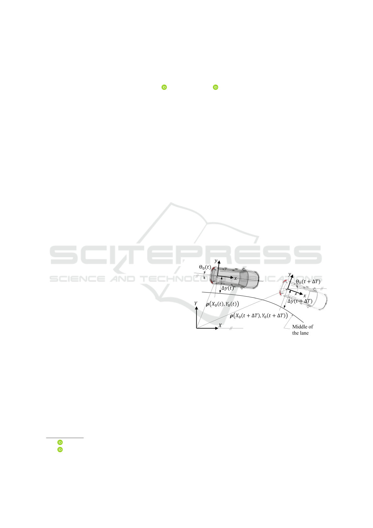
Figure 1: The vehicle coordinate system and the lane offset.

This quantity gives the distance between the centre

of the lane and the origin of the vehicle coordinate

frame, ﬁxed to the rear axle. This frame is a two-

dimensional moving frame in the ﬁxed global frame

deﬁned by



X Y



. The vehicle coordinate frame is

given by ρ



(t) Y

(t)



position vector and Θ

(t)

orientation. An illustration is given in Figure 1. The

lane offset ∆y(t) is the superposition of planning and

execution. Planning is assumed to be slower, with a

longer time horizon, while execution is a short term

process. The following quantities are introduced:

Planned Lane Offset: ∆y

planned

(t)

Offset Error: ∆y

error

(t)

Ignéczi, G., Horváth, E. and Borsos, A.

Analysis of Drivers’ Path Follow Behaviour.

DOI: 10.5220/0012889100003822

Paper published under CC license (CC BY-NC-ND 4.0)

In Proceedings of the 21st International Conference on Informatics in Control, Automation and Robotics (ICINCO 2024) - Volume 2, pages 93-100

ISBN: 978-989-758-717-7; ISSN: 2184-2809

The lane offset is given by the sum of these terms:

∆y(t) = ∆y

planned

(t) + ∆y

error

(t) (1)

The aim is to separate the two components of the lane

offset given in (1). The simple solution is to model

the planned lane offset as the long-term average of

the lane offset. Although for large number of samples

the long term average gives a good estimate of the

expected value of the planned lane offset, for shorter

snippets it is really far from the actual value. This

proves the instinctive idea that drivers change their

planned position in time. It is therefore advisable to

low-pass ﬁlter the lane offset to obtain the planned

lane offset, as given in (2).

∆y

planned

(t) = g

(∆y(t), f

)

∆y

error

(t) = ∆y(t) − ∆y

planned

(t) (2)

where f

is the ﬁlter cut off frequency, g

(∆y(t), f

)

is the low-pass ﬁlter equation. Filtering the lane offset

divides the data into two parts: low frequency changes

in the lane offset, which is the planned lane offset,

and high frequency changes in the lane offset, which

is the offset error. The offset error is the result of the

manoeuvre execution and as such represents a vehicle

level control scheme. This scheme is to be modelled

by observing the behaviour of human drivers.

The problem we wish to analyse in this paper is de-

ﬁned by the following questions:

• Offset error separation: how can we separate the

offset error from the planned lane offset?

• Control scheme modelling: how can we model the

control scheme of a generic driver?

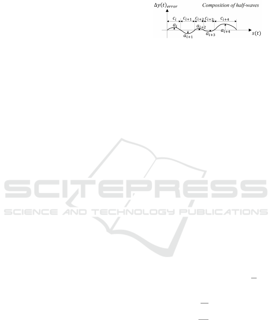
The offset error is expected to be a composi-

tion of half-waves, that represent a drift-away-and-

compensate behaviour. Drift and Compensation in

this context mean a relative movement to the planned

path. During the drift phase, the driver is assumed to

be letting the vehicle go by applying a small amount

of torque to the steering wheel. In the compensation

phase, the driver actively intervenes to compensate

the increased offset error. An illustration is given in

Figure 2. The complete drift and compensation phase

is called snippet. The point between the two phases

is called intervention point. The intervention point is

the time at which the offset error reaches its local ex-

tremum a

= ∆y

extr,i

error











max{∆y

error

(t)}

end,i

start,i

for left side compensation

min{∆y

error

(t)}

end,i

start,i

for right side compensation

(3)

start,i

and t

end,i

are the start and end time points of the

snippet i. In the following we analyse real drivers’

Figure 2: The offset error oscillation schemes, illustrated by

manually drawn signals. The short-term compensation be-

haviour results in oscillating offset error, which is assumed

to be a sequential composition of half-waves of different

frequency and amplitude.

data to determine the cut-off frequency f

given in (2)

and thus to separate the offset error from the planned

lane offset given in (1). Then, the offset error be-

haviour is reproduced using a control driver model. It

is demonstrated that drivers indeed follow the drift-

and-compensate scheme. The results can be used

to design human-like controllers and to better under-

stand human lane-following behaviour.

2 OFFSET ERROR SEPARATION

In this section, the cut-off frequency f

given in (2) is

calculated. A two-step approach is used. First, rec-

ommendations for the value of f

are sought from the

literature. Then, simulations are performed to explore

possible cut-off frequencies, and the ﬁnal value is

chosen. The simulation is done using real-life drivers’

data (Ign

eczi and Horv

ath, 2024). Path-following

driver models are classiﬁed into the following three

groups (Peng, 2005): inverse dynamic models, com-

pensatory models and feedforward models. Inverse

dynamic models usually specify a look-ahead time to

determine control error (Conlter, 1992) (Wang et al.,

2020) (D Salvucci and Gray, 2004) (Erno et al., 2019).

For instance, (Hess and Modjtahedzadeh, 1990) sug-

gests using T

contT heo

= 0.16s to look ahead. (Wang

et al., 2020) suggests a look ahead distance of d

8m at v

= 2m/s, which is equal to T

= 4s.

These look-ahead times are converted to frequency

values:

= 6.25Hz

= 0.25Hz (4)

Compensatory models, such as the Control Theoretic

Model (Hess and Modjtahedzadeh, 1990), divides the

control task into subtasks: vehicle position and actu-

ator control. These two layers are different in which

frequency range they represent the movement of the

vehicle. Actuator control is a high frequency control

scheme, while vehicle position control is modelled

ICINCO 2024 - 21st International Conference on Informatics in Control, Automation and Robotics

as a PI controller in a lower frequency range. The

crossover frequency between these two is suggested

to be 1 rad/s = 0.16 Hz. The time constant of the

PI controller is selected one decimal point below the

crossover frequency, which equals 0.016 Hz. These

together deﬁne the range of the recommended ﬁlter

cut-off frequency:

0.016Hz ≤ f

≤ 0.16Hz (5)

A similar compensation model is developed in (Saleh

et al., 2011). The suggested vehicle position control

time constant is T

= 3s, which equals:

2πT

= 0.053Hz (6)

Note that the time constant is related to the angular

frequency of the system, so multiplication by 2π is

required. Although the frequency characteristics of

the drivers are not speciﬁcally analysed in (D Salvucci

and Gray, 2004), the controller is tuned to oscillate

around the target path with a cycle time of T

= 2s,

then:

= 0.5Hz (7)

Feedforward models use the vehicle model to predict

its behaviour and thus calculate an optimal control tra-

jectory on a so called prediction horizon (McAdam,

1980) (Peng, 2005) (Jiang et al., 2019) (Katriniok

et al., 2013). The prediction horizon length suggested

in (McAdam, 1980) is not speciﬁcally deﬁned, while

in (Jiang et al., 2019) and (Peng, 2005) the horizon is

recommended to be not more than T

mpc,1

= 60s and

between T

min

= 1s and T

max

= 2s respectively. This

can be translated to frequencies:

mpc,1

≥

mpc,1

= 0.016Hz

max

= 0.5Hz ≤ f

mpc,2

≤

min

= 1Hz

(8)

It is clear that the papers do not agree on what is de-

ﬁned as the optimal control frequency. However, they

do give a range of possible frequencies, as given in

(eq:simulationFrequency).

min

min( f

, f

mpc,1

, f

mpc,2

) = 0.016Hz

≤ f

max

max( f

, f

mpc,1

, f

mpc,2

) = 1Hz

(9)

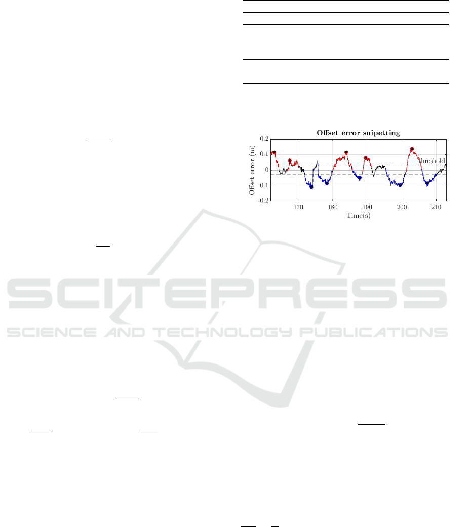
This frequency range is now tested, the test steps are

detailed in Table 1. An example of the snippet is

shown in Figure 3. The threshold is chosen to be 10%

Table 1: Filtering and Snippeting Algorithm.

Step 1: Filtering lane offset using f

Step 2: Offset error calculation given in (2)

Step 3: Thresholding of the offset error

Sections, where the offset error absolute value

is below a small threshold, are neglected

Step 4: Intervention point calculation

The peaks in the offset error are searched

Step 5: Snippetting

The time point when the offset error reaches

zero in time forward and backward are searched

Figure 3: The visualization of snipetting the half-waves

based on the offset error. Blue sections indicate right

side half-waves, red sections indicate left side half-waves.

Source of data: HLB4AV dataset (Ign

eczi and Horv

ath,

2024), driver no. 001.

of the standard deviation of the lane offset. In this

example the cut-off frequency is f

= 0.1Hz.

After ﬁltering and cutting, the snippets are tested

based on performance metrics. Let us take the as-

sumption that the distribution of the length of snippets

from Figure 2 is

∈ N (µ

,σ

) (10)

We aim to minimize σ

. In addition, an indicator of

the coverage of the snippets is calculated. Its formula

is given in (11).

coverage =

∑

i=1

(11)

N is the number of snippets, c

is the length of the

snippet i as shown in Figure 2. T is the total length

of the data. The higher the coverage, the better the

cut. The simulation is run using values of the cut-

off frequency in the range given in (9). The results

are shown in Figure 4. The σ

value has been nor-

malised to its maximum value, namely σ

normalised

max

, in order to have similar scale to the cov-

erage. Also, coverage has been recalculated to har-

monise its interpretation with σ

: the higher σ

, the

worse the performance. Therefore, (1 − coverage) is

plotted instead of coverage. The indicators are cal-

culated individually for all drivers and all f

selec-

tions, then the mean, minimum and maximum per fre-

quency values are plotted. The optimum performance

Analysis of Drivers’ Path Follow Behaviour

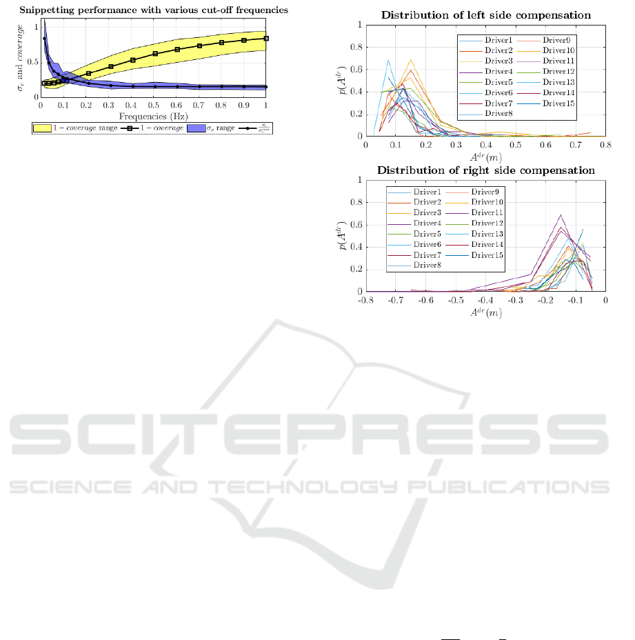
Figure 4: J(F

) cost of various cut-off frequency selection

for all drivers in our dataset (Ign

eczi and Horv

ath, 2024).

is where the mean curves intersect, which fall in the

range of 0.1Hz ≤ f

≤ 0.12Hz. In the followings, the

offset error is calculated by applying (2) with a cut-off

frequency given in (12).

f inal

= f

= 0.11Hz (12)

3 COMPENSATION SCHEME

MODELLING

3.1 Intervention Point Calculation

In Section 2 the ﬁlter cut-off frequency was deﬁned.

The offset error is then cut into snippets using the al-

gorithm introduced in Table 1. In this section, the

snippets are analysed to show how the compensation

behaviour of a generic driver can be modelled. As

shown in Figure 2, a snippet consists of three sections:

drift-away phase, intervention point, and compensa-

tion phase. Based on deﬁnition introduced in (3), let

us denote the set of offset error extrema for a given

driver dr ∈ Dr from driver group Dr with A

= {a

,·· · , a

}

(13)

N is the number of snippets. The snippets are sep-

arated for left and right side deviations. The dis-

tribution of A

le f t

and A

right

for different drivers are

shown in Figure 5. For all drivers a

≥ −0.65m and

≤ 0.65m. However, the probability of such ex-

treme offset error values is small. For most drivers

−0.3m ≤ a

≤ 0.3m. The highest probability (mean

of A

) is in the range of 0.075m ≤ A

≤ 0.15m,

∀dr ∈ Dr for the left deviation and −0.15m ≤ A

≤

−0.05m ∀dr ∈ Dr for the right deviation from the

planned path. In the following sections the values

given in (13) are used for the simulations.

3.2 Control Model

Once the intervention point is calculated, the drift-

away and compensation phases can be separated. An

Figure 5: The distribution of offset error extrema of 15

drivers of the HLB4AV dataset (Ign

eczi and Horv

ath,

2024). Most of the drivers intervene at an offset error be-

tween 0.05 and 0.15 m.

event-based Model Predictive Control (MPC) is set

up, using different weights of its cost function for the

drift and compensation phases. The MPC is based on

a kinematic single-track model, whose equations are

given in (14).

ξ,r

cos(Θ)dτ + X

r,0

ξ,r

sin(Θ)dτ +Y

r,0

ξ,r

dτ + v

ξ,r,0

Θ =

ωdτ + Θ

ω =

ξ,r

= v

ξ,r

tan(δ

)

tan(δ

) = lκ (14)

Where X

and Y

are the global coordinates of the ve-

hicle, Θ is the global orientation, v

ξ,r

and a

ξ,r

are the

speed and acceleration of the vehicle in its own frame,

ω is the yawrate of the vehicle. δ

is the road-wheel-

angle of the front wheel, l is the longitudinal axle dis-

tance, κ is the curvature, ρ is the radius of the vehicle

path. This model is linearized around working point

x =



ξ,r,0



. Then, the linearized

model is used with the MPC structure proposed by (L,

2009). During drifting, the vehicle is released by ap-

plying a small amount of torque to the steering wheel

to meet the driver’s comfort requirements (no active

ICINCO 2024 - 21st International Conference on Informatics in Control, Automation and Robotics

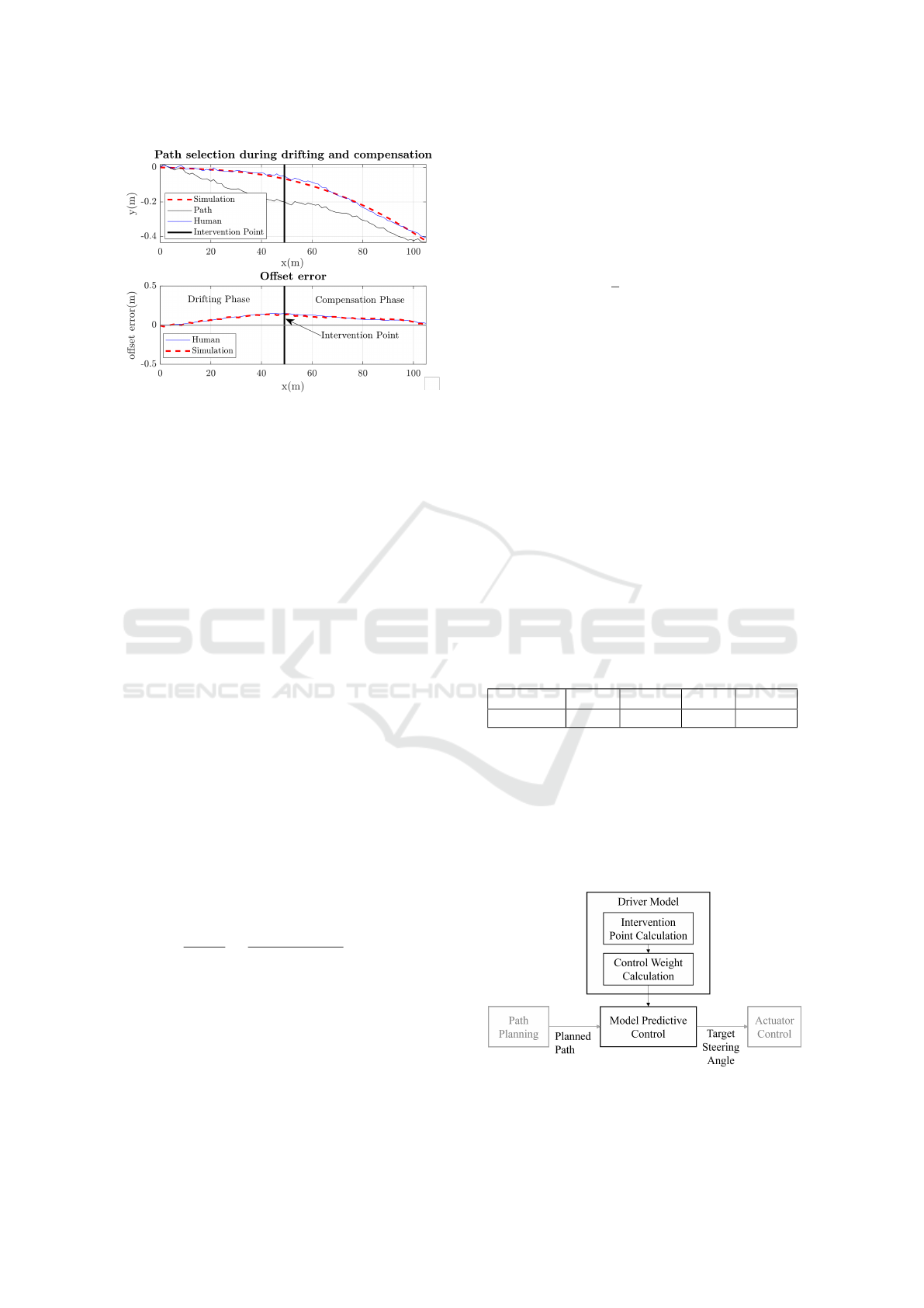
Figure 6: Examples of snippets from data of driver no. 001

from HLB4AV dataset (Ign

eczi and Horv

ath, 2024). Blue

lines are directly from the measurement, red lines are res-

imulated signals using the MPC logic.

control is required). As soon as the driver judges the

situation to be critical, high steering torque is applied

to compensate for the offset error and return the vehi-

cle to the planned path, satisfying the driver’s risk re-

duction requirement. These two opposing control tar-

gets are included in most MPC cost functions (Peng,

2005) (Jiang et al., 2019) (McAdam, 1980) (Katriniok

et al., 2013). The cost function is deﬁned as

J(∆U

U,E

E) =

∑

n=1

∆U

R∆U

U +E

E (15)

where ∆U

U ∈ R

N×N

is a matrix of input signals, N

is the number of inputs, N

is the prediction hori-

zon, E

E ∈ R

M×N

is a matrix of output errors, M is

the number of outputs, R

R ∈ R

M×M

and Q

Q ∈ R

N×N

are

weight matrices. In our application, the input signal

is the steering wheel angle, while the output error is

the offset error. There are ﬁve parameters in this MPC

conﬁguration: the steering wheel amplitude and off-

set error weights for the drift-away and compensation

phases, w

and w

, w

and w

respectively, and the

prediction horizon N

. The prediction horizon is cho-

sen based on the offset error cut-off frequency given

in (12):

× T

0.11Hz × 0.05s

≈ 180 (16)

where T

is the measurement sampling time. By

choosing the weights correctly, the drift-away and

compensation paths can be reproduced. The follow-

ing steps are performed:

1. the data of the given driver is cut to snippets,

2. the intervention points given in (13) are calculated

based on (3),

3. the MPC weights of the drift-away and compen-

sation phases are optimized by simulating the ve-

hicle path based on (17).

The optimization is done using the fmincon function

of MATLAB. The optimization problem is deﬁned as

follows:

min

∆y

error

(t, w

)dt

s.t. w

≥ 0 (17)

where t

is the end of the compensation phase, t

the start of the drift phase, ε

∆y

error

(t)

is the output error

calculated according to (18).

∆y

error

(t, w

) =



∆y

error,sim

(t, ·)− ∆y

error,meas

(t, ·)



(18)

An example of resimulation using the optimised

weights for Driver 001 (Ign

eczi and Horv

ath, 2024)

are shown in Figure 6. In simulation, the controller

output is applied on the model introduced in (14). The

model and the controller are implemented in MAT-

LAB. The event-based MPC succeeds to reproduce

the drift and compensation path. The weights for

these two snippets are shown in Table 2. The overall

results for all drivers are given later in Section 4. We

Table 2: The optimized parameters of Driver 1 for the snip-

pet, shown in Figure 6.

Snippet 1 0.007 32.366 0.003 65.802

propose to use the model structure shown in Figure 7.

The MPC block acts as the vehicle level control, cal-

culating the target steering angle based on the planned

path. The controller dynamics are inﬂuenced by the

controller parameters provided by the Driver Model.

It includes the intervention point calculation and the

controller parameter calculation.

Figure 7: The proposed model structure.

This driver model structure is used to generate the

Analysis of Drivers’ Path Follow Behaviour

overall results. The intervention point is calculated

from the measurements using the values shown in

Figure 5. The MPC weights are taken from the re-

sults of the optimisation introduced in (17).

4 RESULTS

In this section the driver model is used together with

the MPC from Figure 7 to simulate vehicle paths.

The planned path is based on the planned lane offset

∆y

planned

(t) from (1). The goodness of the model is

given by the Normalised Root-Mean-Square (NRMS)

value of the Euler distance (ED) between the sim-

ulated path and the measured path. The simulated

path is interpolated for the longitudinal coordinates

x of the measured path. Therefore, the Euler dis-

tance of the path points are simpliﬁed to the differ-

ence between the y coordinates (note that the x co-

ordinates are strictly monotonically increasing in all

cases). The ED vector for the i

section is calculated

as follows:

= ∥P

sim

− P

meas

∥ =



sim

− y

meas



(19)

where P

sim

∈ R

M×2

and P

meas

∈ R

M×2

are the 2D co-

ordinates of the simulated and measured paths respec-

tively. Similarly, y

sim

and y

meas

are the y coordinates

of the simulated and measured paths respectively. M

is the number of sample points in the snippet. Also

∈ R

. Then the NRMS value of the vector E

is calculated. The normalisation is done using the

range of E

NRMS

(

∑

j=1

[ j]

)

max(E

) − min(E

)

(20)

where j is a running index indicating the j

element

of E

vector. Finally, the mean and standard devi-

ation of the NRMS

values of the given driver are

calculated:

NRMS

∑

i=1

NRMS

(21)

NRMS

∑

i=1

(NRMS

−

NRMS

)

(22)

where S is the number of snippets in the measurement

of driver dr. This indicator is calculated for all left

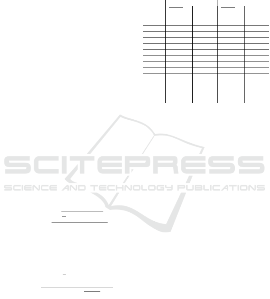
and right snippets, separately. The result of all test

drivers are shown in Table 3. The NRMS value gives a

ratio between the total error and the quantity in focus.

Thus, an error of 0.017 (as in the case of Driver 1)

means that the average distance of the simulated path

Table 3: Results of the simulations. The NRMS value of

the distance between planned and measured path. Source of

data: (Ign

eczi and Horv

ath, 2024).

Left deviation Right deviation

Dr NRMS

NRMS

Dr001 0.017 0.019 0.011 0.013

Dr002 0.019 0.024 0.008 0.010

Dr003 0.013 0.013 0.015 0.021

Dr004 0.052 0.044 0.026 0.085

Dr005 0.034 0.056 0.030 0.027

Dr006 0.018 0.025 0.045 0.058

Dr007 0.279 0.764 0.032 0.029

Dr008 0.016 0.033 0.175 0.575

Dr009 0.022 0.030 0.018 0.020

Dr010 0.022 0.030 0.039 0.051

Dr011 0.016 0.019 0.027 0.034

Dr012 0.022 0.026 0.032 0.048

Dr013 0.037 0.066 0.038 0.056

Dr014 0.018 0.024 0.026 0.031

Dr015 0.022 0.029 0.054 0.153

from the measured one is the 1.7% of the range of the

measured y coordinates. In this sense, the comparison

is intuitively easy. The mean and standard deviation

of NRMS

are in most cases less than 10%. The

error is slightly higher in the case of Driver 7 (mean is

around 28%). The analysis of Driver 7’s data showed

that in certain cases the MPC reacts more dynamically

in the compensation phase of this driver. We believe

that the problem may be caused by optimiser ﬁnding a

local minimum instead of the global one, as the shape

of the offset error is very similar to other drivers.

5 CONCLUSIONS

In this paper we have investigated the compensatory

behaviour of human drivers around their planned

path. The offset signal to the lane centre was ﬁl-

tered, resulting in the offset error signal. We expected

drivers to oscillate continuously around their planned

path, ﬁrst drifting away from it (increasing offset er-

ror), then intervening and compensating the increased

error back to zero towards the planned path (decreas-

ing offset error). This is called as the drift-away

and compensate behaviour. The proposed solution

provides not only a control algorithm (this is taken

over from the state-of-the-art Model Predictive Con-

trollers), but the parametrization, as well. It means,

that using MPCs with the proposed driver parameters

the output of the closed loop control will be closely

human-like. Such analysis is rarely executed in the

ﬁeld of vehicle controls, as the requirements used in

similar papers focus on minimizing the error to a pri-

orly planned path (e.g., midlane). However, this is

often unnaturalistic, as people wish to deviate from

the midlane.

ICINCO 2024 - 21st International Conference on Informatics in Control, Automation and Robotics

In this paper it was shown that a suitable low pass

ﬁlter frequency is f

= 0.11Hz. The offset error sig-

nal was decomposed into half-waves, which account

for the full drift and compensate snippets. It has been

shown, that the total length of these snippets is about

80% of the full data length, proving the generality of

the ﬁltering and cutting. Secondly, the intervention

point when the driver switches from the drift to the

compensation phase was calculated. The offset error

extrema associated with the intervention are between

0.05m and 0.15m for most of the drivers. Thirdly,

the drift and compensation phases have been mod-

elled using an event-based Model Predictive Control

(MPC), with different weights for the two phases. The

values of these weights were calculated by optimis-

ing the model output against the drivers’ measure-

ments. Finally, it has been demonstrated that the pro-

posed driver model together with the MPC can ac-

curately reproduce the compensation path of the se-

lected drivers.

These results provide better understanding of the

drivers’ path following behaviour. Usually, the re-

sulting vehicle path can be measured (e.g., with ac-

curate GPS), which is the result of the driver’s de-

tection, perception, planning and control behaviour,

together. The environmental inputs, such as the po-

sition of the road edge or other objects, can also be

measured. However, the layers in between cannot be

observed properly from a single sequence of data. By

modelling the drift-away and compensation path, the

vehicle level compensation can be ﬁltered out of the

measured data sequence. This enables the estimation

of the planned lane offset, and contributes to a more

accurate validation of driver models at the path plan-

ning level.

The drift-away and compensation model also con-

tributes to the design of a lane-keeping system with

human-like characteristics. Although the underly-

ing controllers are usually designed to give the best

path accuracy, another possibility is to mimic human

steering characteristics. This can contribute to an in-

creased level of trust in such driving systems. The

results of this paper give important inputs to achieve

more human-like lane following behaviour, on the

other hand requires further analysis with the inclusion

of other domains, such as path planning and actuator

control. We believe that an interesting next research

topic is to build predictive driver models, that enable

the intervention point and the compensation dynam-

ics to be calculated at runtime. It would also be an

exciting challenge to analyse the model parameters

for each driver and ﬁnd ways to cluster them based

on these parameters.

While the results presented in this paper are

promising and validate the concept on a sample

dataset, these results are limited in their applicabil-

ity. Firstly, the number of drivers tested is limited by

the size of the dataset. Therefore, it is not yet proven

whether the concept is generic to a wider range of

drivers. Secondly, the results are generated by simu-

lation and vehicle control algorithms, such as MPCs,

are very sensitive to real-world conditions (e.g. ac-

curacy of the vehicle model). This may hinder the

realisation of the proposed algorithm.

ACKNOWLEDGEMENT

The research was supported by the European Union

within the framework of the National Laboratory for

Autonomous Systems. (RRF-2.3.1-21-2022-00002).

REFERENCES

Cody, D. and Gordon, T. (2007). Trb workshop on driver

models: A step towards a comprehensive model of

driving? Modelling Driver Behaviour in Automotive

Environments, 1(1):26–42.

Conlter, R. C. (1992). Implementation of the pure pursuit

path tracking algorithm.

D Salvucci, D. and Gray, R. (2004). A two-point visual

control model of steering. Perception, 33(1):1233–

1248.

Erno, H., Csaba, H., and Peter, K. (2019). Novel pure-

pursuit trajectory following approaches and their prac-

tical applications. In Proceedings of the 10th IEEE

International Conference on Cognitive Infocommuni-

cations, pages 1–6, Naples, Italy.

Evans, L. and Schwig, R. C. (1985). Human behavior and

trafﬁc safety. Plenum Press, New York, NY.

Hess, R. and Modjtahedzadeh, A. (1990). A control theo-

retic model of driver steering behavior. IEEE Control

Systems Magazine, 10(5):3–8.

Ign

eczi, G. and Horv

ath, E. (19-21, September 2024).

Human-like behaviour for automated vehicles

(hlb4av) naturalistic driving dataset, data available at

https://jkk-research.github.io/dataset/jkk dataset 03/.

In IEEE 22nd International Symposium on Intelligent

Systems and Informatics (SISY 2024), Pula, Croatia.

Jiang, H., Tian, H., and Hua, Y. (2019). Model predictive

driver model considering the steering characteristics

of the skilled drivers. Advances in Mechanical Engi-

neering, 11(3):1–14.

Katriniok, A., Maschuw, J. P., et al. (2013). Optimal vehi-

cle dynamics control for combined longitudinal and

lateral autonomous vehicle guidance. In Proceed-

ings of European Control Conference, pages 974–979,

urich, Switzerland.

Klebersberg, D. (1971). Subjektive und objektive sicherheit

im strassenverkehr als aufgabe f

ur die verkehrssicher-

Analysis of Drivers’ Path Follow Behaviour

heitsarbeit. Schriftenreihe der Deutschen Verkehr-

swacht, 1(5):3–12.

L, W. (2009). Model Predictive Control System Design and

Implementation using Matlab. Springer, Verlag.

McAdam, C. C. (1980). An optimal preview control for lin-

ear systems. Journal of Dynamic Systems, Measure-

ment and Control, 102(1):188–190.

McKnight, J. A. and Adams, B. B. (1970). Driver Educa-

tion Task Analysis. Human Resources Research Or-

ganisation, Alexandria, Va.

Michon, J. A. (1985). A Critical View of Driver Behavior

Models: What do we know, what should we do? Uni-

versity of Groningen, The Netherlands.

Peng, H. (2005). An adaptive lateral preview driver model.

Vehicle System Dynamics, 1(1):1–17.

Saleh, L., Philippe, C., Mars, F., et al. (2011). Human-

like cybernetic driver model for lane keeping. In Pro-

ceedings of the International Federation of Automatic

Control, pages 4368–4373, Milano, Italy.

Theeuwes, J. (1993). Visual selective attention: a theoreti-

cal analysis. Acta Psychologica, 83(2):93–154.

Wang, R., Li, Y., et al. (2020). A novel pure pur-

suit algorithm for autonomous vehicles based on salp

swarm algorithm and velocity controller. IEEE Ac-

cess, 1(1):166525–166540.

W.H, J. (1979). Routeplanning en geleiding: Een literatu-

urstudie. Report IZF. C-13. Soesterberg (The Nether-

lands): Institute for Perception TNO.

Wilde, G. J. S. (1982). The theory of risk homeostasis:

Implications for safety and health. Risk Analysis,

2(4):209–225.

ICINCO 2024 - 21st International Conference on Informatics in Control, Automation and Robotics

100