MLN-Subdue: Substructure Discovery In Homogeneous Multilayer

Networks

Anish Rai, Anamitra Roy, Abhishek Santra and Sharma Chakravarthy

Computer Science and Engineering Department and Information Technology Laboratory (IT Lab),

The University of Texas at Arlington, Arlington, Texas 76019, U.S.A.

{anish.rai, axr9563, abhishek.santra}@mavs.uta.edu, sharmac@cse.uta.edu

Keywords:

Multilayer Networks, Substructure Discovery, Decoupling Approach, Map/Reduce Architecture.

Abstract:

Substructure discovery is a well-researched problem for graphs (both simple and attributed) for knowledge dis-

covery. Recently, multilayer networks (or MLNs) have been shown to be better suited for modeling complex

datasets that have multiple entity and relationship types. However, the MLN representation brings new chal-

lenges in ﬁnding substructures due to the presence of layers, and substructure discovery methods for MLNs

are currently not available.

This paper proposes a substructure discovery algorithm for homogeneous MLNs using the decoupling ap-

proach. In HoMLNs, each layer has same or a common subset of nodes but different intralayer connectivity.

This algorithm has been implemented using the Map/Reduce framework to handle arbitrarily large layers and

to improve the response time through distributed and parallel processing. In the decoupled approach, each

layer is processed independently (without using any information from other layers) and in parallel and the

substructures generated from each layer are combined after each iteration to generate substructures that span

layers. The focus is on the correctness of the algorithm and resource utilization based on the number of layers.

The proposed algorithm is validated through extensive experimental analysis on large real-world and synthetic

graphs with diverse graph characteristics.

1 MOTIVATION

Mining has been traditionally performed on transac-

tional data whether it is clustering, classiﬁcation, or

identifying frequent itemsets. For applications where

there is an inherent relationship, graphs offer better

representation for the modeling of data. As a result,

mining techniques were extended to graph models.

Graphs can also be used to model relationships among

multiple object types and relationships in a variety of

applications such as chemical compounds, virus prop-

agation, electrical and road transportation networks,

web analysis, etc. In particular, with graph models

where each vertex corresponds to an entity and each

edge corresponds to a relationship between two enti-

ties, the problem of ﬁnding frequent patterns becomes

one of discovering subgraphs that occur frequently or

compress the graph or forest better.

Substructure discovery (Cook and Holder, 1993)

was developed as a main memory algorithm for graph

models when data sizes were not very large. However,

with the advent of social networks and the Internet,

graph sizes have grown signiﬁcantly, necessitating al-

ternative approaches to substructure discovery.

Why Multilayer Networks (MLNs)? As graphs be-

come larger (in terms of the number of nodes and

edges) and complex (in terms of the number of en-

tity types and relationships), modeling the data using

a representation that preserves the structure and se-

mantics of data becomes important. A model that is

also amenable to efﬁcient analysis is another issue to

reckon with. From these perspectives, MLNs offer

distinct advantages.

Simple graphs are unable to capture the complex-

ity of data and its semantics although a large num-

ber of analysis algorithms exist for them. Attributed

graphs can handle additional complexity with multi-

ple edges, but lack analysis algorithms. MLNs, as a

network of networks, offer separation of semantics (as

individual layers) and ﬂexibility of analysis (when de-

coupling approach (Santra et al., 2017b; Santra et al.,

2017a) is used) using desired subsets of layers. In ad-

dition, extant simple graph analysis algorithms can be

leveraged in the decoupling approach.

If MLNs are used for modeling, each layer in the

MLN represents a different relationship, either be-

Rai, A., Roy, A., Santra, A. and Chakravarthy, S.

MLN-Subdue: Substructure Discovery In Homogeneous Multilayer Networks.

DOI: 10.5220/0012906200003838

Paper published under CC license (CC BY-NC-ND 4.0)

In Proceedings of the 16th International Joint Conference on Knowledge Discovery, Knowledge Engineering and Knowledge Management (IC3K 2024) - Volume 1: KDIR, pages 36-47

ISBN: 978-989-758-716-0; ISSN: 2184-3228

tween the same type of entities within a layer (in-

tralayer edges), or across layers between different

types of entities (interlayer edges). The advantages

of modeling data using MLNs are discussed in (Boc-

caletti et al., 2014; Santra et al., 2017b; Kivel

a et al.,

2013). However, with the use of MLNs, the challenge

is to extend graph analysis algorithms, be it commu-

nity, centrality, or substructure detection, to the new

representation.

Depending on the types of entities, multiple layers

can be deﬁned for the same (or a subset of) entity type

or different entity types. MLNs can be of three dif-

ferent types: Homogeneous, Heterogeneous, and Hy-

brid. Homogeneous Multilayer Networks (HoMLNs)

are used to model multiple distinct relationships ex-

isting between the same type of entities. Each set of

intralayer edges represent one particular type of re-

lationship, and the interlayer edge sets are implicit,

as the same set of nodes are present in every layer.

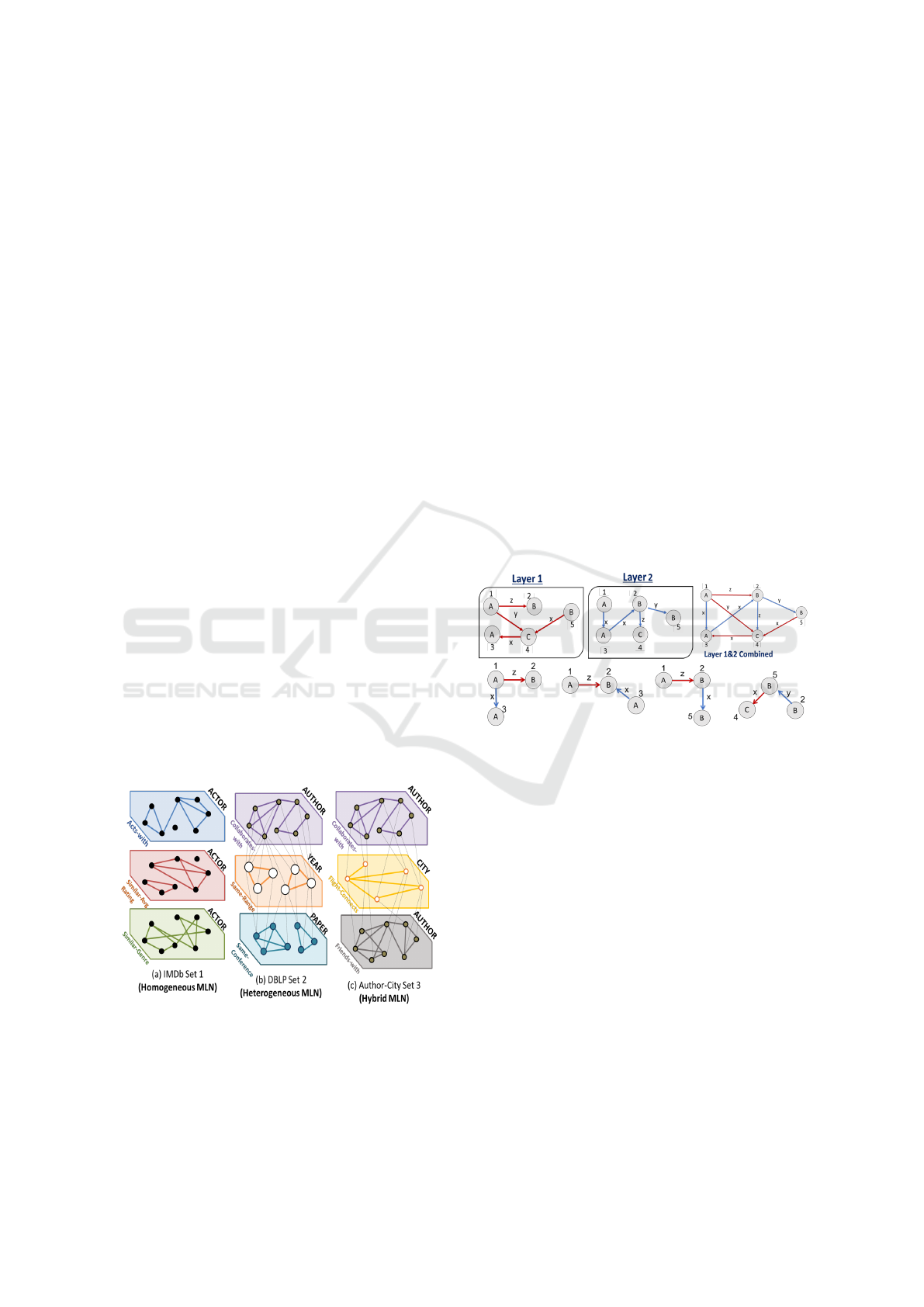
For example, the same set of actors can be connected

based on co-acting, similar average rating, and similar

movie genres they work in forming three different lay-

ers as shown in Figure 1 (a). Relationships among dif-

ferent types of entities are modeled through Heteroge-

neous Multilayer Networks (or HeMLNs), as shown

in Figure 1 (b). The interlayer edges here are explic-

itly represented to demonstrate the relationship across

layers. For example, there can be edges between the

author layer and paper layer, if an author has writ-

ten that paper. Finally, for data that includes multi-

ple relationships within and across different types of

entity sets, a combination of homogeneous and het-

erogeneous multilayer networks can be used, called

Hybrid Multilayer Networks (or HyMLNs), as shown

in Figure 1 (c).

Figure 1: Examples of MLN Types.

Why Map/Reduce? We have used the Map/Reduce

paradigm as an example of the distributed and parallel

processing approach. Without loss of generality, any

other paradigm (e.g., Spark) can be used in its stead

without modifying the overall approach.

Problem Statement: The problem addressed in this

paper is ﬁnding interesting and frequent substruc-

tures in a given Homogeneous Multilayer Network

(HoMLN) using the decoupling approach proposed

in (Santra et al., 2017a; Santra et al., 2017b; Santra

et al., 2022) to leverage its advantages. This amounts

to not converting the MLN into a single graph, but still

getting the same result as if the MLN was processed

as a single graph.

The main challenge here is to use the substruc-

tures generated for each layer independently and in

parallel to compose them to compute the missing sub-

structures that span multiple layers correctly and ef-

ﬁciently. To the best of our knowledge, there are

no MLN substructure discovery algorithms. How-

ever, the rationale for using the decoupling approach

is that existing algorithms from the literature(Cook

and Holder, 1993; Das and Chakravarthy, 2015) can

be used effectively for each layer. When these algo-

rithms are used to ﬁnd substructures in each layer in-

dependently, many substructures that span layers will

be missing as shown in Figure 2.

Figure 2: Substructures that span layers - only combined

graph can generate them (color coded).

Approaches for MLN Substructure Discovery:

MLNs can be processed for various types of analyses

(community detection, substructure discovery etc.)

Alternative approaches are listed below with a brief

explanation.

1. Traditional Aggregation Approach: In this ap-

proach, layers of a MLN are conﬂated into a single

graph. Boolean AND or OR aggregation can be used

to reduce a HoMLN to a simple graph and ﬁnd sub-

structures correctly for a given multilayer network.

The aggregation process can be costly (depending on

the number of layers) and the resulting graph can be

large (for OR composition). As a result, substructure

discovery time can be signiﬁcantly greater than that of

a single layer. This approach also restricts paralleliza-

tion as each layer cannot be processed in parallel. The

loss in MLN structure, due to aggregation, also makes

it difﬁcult to drill-down results without maintaining

MLN-Subdue: Substructure Discovery In Homogeneous Multilayer Networks

extensive mapping. Finally, for processing a subset of

layers, separate aggregation is required – making the

approach less ﬂexible and inefﬁcient.

2. Decoupling-Based Approach: It is a “divide

and conquer” approach for analyzing multilayer net-

works. The goal is to ﬁnd substructures in each layer

independently and then use a separate composition

function to combine the results to generate what is

missing for that analysis (e.g., community, central-

ity, substructure, motif, etc.) The decoupling-based

approach used in this paper to address the substruc-

ture discovery problem is described along with a ﬁg-

ure (Figure 5) in Section 4.

3. Holistic Approach: In this approach, neither the

MLN is aggregated nor the decoupling approach is

used. An algorithm is developed from scratch (as

available graph analysis algorithms cannot be used as

in the previous two approaches), keeping the struc-

ture and semantics intact. However, a new algorithm

need to be developed for each analysis making this

approach complex as the algorithm needs to traverse

back and forth across layers. This approach has been

used for coherent clusering in (Boden et al., 2012)

We use the decoupling-based approach in this pa-

per as it is efﬁcient and extant analysis algorithms

(there are several of them depending on the analy-

sis) can be used. The main challenge to be addressed

is the development of the composition function and

establishing its correctness (soundness and complete-

ness.) Also, evaluating the efﬁciency of this approach

as compared to the aggregation approach (used as GT

or ground truth for validation.)

The contributions of this paper are:

• Adapting the decoupling approach for substruc-

ture discovery

• Developing Map/Reduce approach for substruc-

ture discovery

• Composition algorithm for HoMLN substruc-

ture discovery

• Establishing the empirical correctness of the

composition algorithm

• Extensive experimental analysis with diverse

synthetic and real-world datasets

This paper is organized as follows. Section 2 dis-

cusses related work. Section 3 discusses the prelimi-

naries for substructure discovery using Map/Reduce.

Section 4 details the adaptation of the decoupling

approach for iteration-based substructure discovery.

Section 5 discusses the composition algorithm and

its correctness. Section 6 discusses the Map/Reduce

approach for distributed and parallel computation on

MLN. Section 7 provides experimental analysis. Con-

clusions are in Section 8.

2 RELATED WORK

SUBDUE (Cook and Holder, 1993; Ketkar et al.,

2005) was developed as a main-memory substruc-

ture discovery algorithm. It performs a computa-

tionally constrained beam search where substructures

of increasing size are generated iteratively and eval-

uated using the Minimum Description Length (or

MDL) (Rao and Lu, 1992) metric. The algorithm be-

gins with all substructures of size one (i.e., an edge),

and in each iteration expands the instances by one

neighboring edge in all possible ways. After each it-

eration, the top beam (parameter speciﬁed) substruc-

tures are carried over to the next iteration. Best sub-

structures are output based on the size and other pa-

rameters speciﬁed.

Due to the limitations of the main-memory ap-

proach, the disk-based approach (Wang et al., 2005)

stores the data on disks and stages chunks of data

to memory as needed. The graph is indexed to

speed up retrieval. However, this approach needs

to marshal data between the disk and main memory

buffer, and its performance can be very sensitive to

buffer size, replacement policies, hit ratios, etc. To

overcome the pitfalls of the disk-based approach, a

database management system (or DBMS) was used

to store the graph and SQL for substructure discov-

ery(Padmanabhan and Chakravarthy, 2009). This

takes advantage of the buffer management and opti-

mization provided by the DBMS. Although scalabil-

ity was achieved to graphs of over a million nodes

and edges, use of self-joins on large relations for sub-

structure expansion seems to have made it difﬁcult to

go beyond due to computation resulting in unaccept-

able response time. Also, it appears that the removal

of duplicate substructures required sorting columns in

row-based Relational DBMS, making it expensive in

terms of the number of joins needed.

As the graph sizes grew further with the advent

of social networks and the Internet, graphs had to be

partitioned to deal with the increasing sizes. As a

result scalable parallel computing algorithms had to

be developed. Map/Reduce (Das and Chakravarthy,

2015; Das and Chakravarthy, 2018) and other archi-

tectures were used to address the problem of substruc-

ture discovery on a large graph by dividing the graph

into smaller partitions and then combining the results

across partitions. In addition to substructure discov-

ery, partitioning of graphs has been explored in other

KDIR 2024 - 16th International Conference on Knowledge Discovery and Information Retrieval

research as well (Yang et al., 2012).

With multilayer networks being used for modeling

large complex datasets, there is a need for substruc-

ture discovery algorithms on MLNs. A clustering al-

gorithm (Boden et al., 2012) for ﬁnding clusters in a

multilayer graph has been proposed using the holis-

tic approach described earlier. Similarly, another al-

gorithm (Liu and Wong, 2008) has been proposed to

ﬁnd quasi-cliques to ﬁnd all one-dimensional clusters

in a single layer, which are then used to ﬁnd multi-

dimensional clusters. The focus of this work is to

ﬁnd clusters of vertices that are densely connected by

edges with similar edge labels in a subset of graph

layers.

This paper differs from the above in that we

are proposing a decoupling-based algorithm for sub-

structure discovery that gives the same results as the

ground truth. It is also efﬁcient as compared with the

algorithm used for GT. Further, it uses Map/Reduce

to process each layer and for composition providing

better scalability than extant approaches.

3 TERMINOLOGY USED

Graphs are input as text ﬁles and this section indicates

input formats for MLN-Subdue as well as some termi-

nology needed for understanding the paper.

Input Graph Representation: For substructure dis-

covery, labeled graphs are used where vertex and edge

labels are not assumed to be unique, but all vertex

IDs are unique. The input graph is represented as

an unordered list of 1-edge substructures where each

edge is represented as a 5-element tuple <edge label,

source vertex id, source vertex label, destination ver-

tex id, destination vertex label>. The input graph is

stored in an ASCII ﬁle with a 1-edge substructure in

each line. If needed, graphs in other formats are con-

verted to this format.

Adjacency List: Adjacency list of a vertex ID is the

set of edges that are incident (both outgoing and in-

coming) on that vertex ID. The adjacency list is used

to expand a substructure from each vertex ID in that

substructure using an edge from the adjacency list.

Each 1-edge expansion becomes a separate substruc-

ture. This allows an n-edge substructure to be ex-

panded into a number of (n+1)-edge substructures in

an iteration.

Substructure Expansion: Starting from 1-edge, sub-

structures of increasing size are generated systemati-

cally in each iteration using the adjacency list. As

the goal is to discover interesting substructures of any

size, systematic graph expansion is critical to the pro-

cess. Expansion is done on each substructure inde-

pendently as indicated above. Expansion is uncon-

strained, i.e., each substructure independently grows

into a number of larger substructures in each iteration.

This independent expansion leads to the generation of

duplicate substructures which must be removed to en-

sure correctness. A substructure is represented as a

(lexicographically) ordered list of edges.

Canonical Instances for Duplicate Elimination:

Lexicographic ordering of edges in a substructure is

used to identify duplicates. Each edge in a substruc-

ture is ordered based on edge label, then source vertex

label, then destination vertex label, and ﬁnally source

and destination vertex IDs. If any of the values match,

the comparison moves forward to the next compo-

nent, else the ordering is performed. A substructure

can be uniquely represented using the lexicographic

order of 1-edge components. This is called a canoni-

cal k-edge instance. Intuitively, two duplicate k-edge

substructures must have the same ordering of labels

and vertex IDs when converted to canonical k-edge

instance

. Figure 3 shows an example of duplicate

substructures generated by two different substructure

instances during independent expansion and how they

are detected as duplicates using their canonical in-

stances.

Canonical Substructures for Graph Isomorphism:

Isomorphs in a graph have the same graph structure

in terms of vertex and edge labels as well as connec-

tivity, but differ in vertex IDs. In contrast, duplicates

have the same vertex IDs. After duplicate elimina-

tion, we need to identify isomorphs to count their oc-

currences. We need to convert canonical instances of

substructures to canonical substructures using rela-

tive ordering of vertex IDs. Intuitively, in the canoni-

cal form, two isomorphic substructures have the same

relative ordering of vertex numbers. To identify

isomorphs, the canonical instance is converted into

a canonical substructure. This is done by replacing

each vertex ID with their relative positions in the in-

stance starting from 1. The inclusion of these relative

positions is critical for differentiating the connectivity

of the instances. Figure 4 shows an example of how

canonical substructure is created from the canonical

instance. It can be seen that the isomorphs have differ-

ent canonical instances. Using the above technique,

the relative positioning of vertex Ids (2, 5, 4) for the

canonical instance 1 and (7, 10, 9) for the canonical

instance 2 are converted to (1, 2, 3). Hence we can

Substructures and substructures instances are used in-

terchangeably when the meaning is clear from the context.

However, substructure instances are converted into rela-

tive ordering of vertex IDs, termed canonical substructures,

which are used for detecting substructure isomorphs.

MLN-Subdue: Substructure Discovery In Homogeneous Multilayer Networks

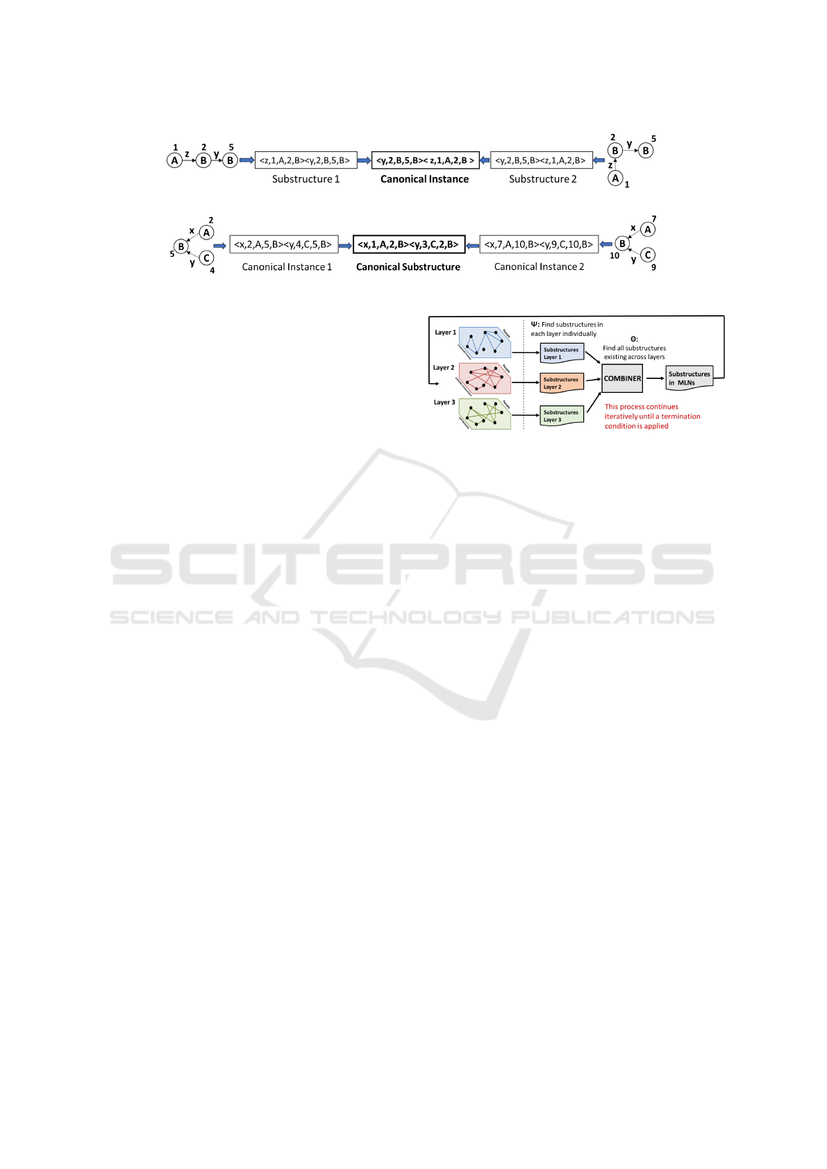
Figure 3: Duplicate substructure identiﬁcation using canonical instances.

Figure 4: Graph isomorphism and canonical substructures.

identify isomorphs using canonical substructures.

Metrics for Ranking: Many metrics are used to

rank substructures based on isomorphs. Frequency of

isomorphic substructures is one such metric (higher

the frequency, the better the substructure.) Another

widely used information-theoretic metric is the Min-

imum Description Length (or MDL (Rao and Lu,

1992)). MDL calculates the importance of a substruc-

ture on how well it compresses the entire graph/forest.

A substructure that compresses the graph better is

considered an interesting and repetitive substructure.

When MDL is used, an MRN (Most Restrictive

Node)(Bringmann and Nijssen, 2008; Elseidy et al.,

2014) metric is used to count non-overlapping in-

stances. But overlapping instances have also been

used to compute frequency and MDL for each sub-

structure.

4 DECOUPLING APPROACH

Multilayer networks consist of multiple layers of sim-

ple graphs where each layer represents a relationship

between entities in that graph. However, most algo-

rithms convert a MLN (or a subset of it) into a sim-

ple graph using aggregation (Domenico et al., 2014)

and/or projection techniques (Berenstein et al., 2016)

to use extant algorithms. However, this leads to loss

of structure, semantics, and information from the ﬁ-

nal analysis results (Kivel

a et al., 2013; De Domenico

et al., 2014). For the other end, existing single

graph algorithms cannot be directly used for the holis-

tic approach described earlier. In this paper, the

decoupling-based approach has been used which pre-

serves the structure and semantics of MLNs (Santra

et al., 2017a; Pavel et al., 2023) while performing

analysis on complex datasets without losing any infor-

mation. It is also shown to be efﬁcient (Santra et al.,

2017a).

The network decoupling approach has been il-

lustrated with respect to substructure discovery in

HoMLNs (focus of the paper) in Figure 5, where each

Figure 5: Substructure Discovery: Decoupling Approach.

layer has the same set of nodes but different edge

connectivity. It consists of two functions: analysis

(Ψ) and composition (Θ). Using the analysis func-

tion, each layer in the network is analyzed indepen-

dently (and in parallel) to obtain the layer substruc-

tures. Then, the partial results from any two (or more)

layers are combined and processed by the composi-

tion function to produce substructures that span par-

ticipating layers. This is done for each iteration as

substructure discovery is an iterative algorithm. This

composition can be binary or n-ary. If binary, it can be

repetitively applied to n layers using previously gen-

erated results. This approach allows parallel analy-

sis of each layer to improve efﬁciency (Santra et al.,

2017a). Further, due to the layer-wise analysis, each

graph is likely to be small, which requires less mem-

ory for computing layer-wise results. Each layer is

also analyzed only once, and the existing single graph

algorithms can be used for that. The results obtained

are then used by the composition function. In addi-

tion, this approach is application-independent.

In this approach, the major challenge is to de-

velop the composition algorithm (Ψ) which is sound

and complete in generating missing substructures that

span layers. It is known from earlier work that sub-

structure generation in each layer is sound and com-

plete.

5 ALGORITHM DESIGN

Substructure discovery in single (simple and at-

tributed) graphs is an iterative process, where inter-

KDIR 2024 - 16th International Conference on Knowledge Discovery and Information Retrieval

Algorithm 1 : MLN-Subdue: Substructure Discovery Al-

gorithm for Homogeneous Multilayer Networks.

Require:

Input: Substructures of size k for k

iteration

Output: Top beam substructures (intralayer & inter-

layer) of size k+1

1: Load Adjacency list for each layer

2: for each substructure of size k in MLN:

3: Expand each k-edge substructure by one edge in all

directions in each layer

4: Eliminate Duplicates using canonical representa-

tion in each layer

5: end for

6: for each expanded k + 1 edge substructure:

7: Group all the expanded substructures from each

layer based on vertex ID

8: Apply Combine-MLN recursive function to form

k + 1 edge interlayer substructures from k+1 edge in-

tralayer substructures

9: Eliminate duplicates generated during combination

10: end for

11: for all the canonical instances in the MLN:

12: Count the frequency of all substructures using iso-

morphism

13: end for

14: Apply metric Frequency or MDL

15: Apply beam heuristic to determine top-beam sub-

structures and send their instances to be used the next

iteration // Specify beam as required

16: Increment k by 1 for next iteration

17: Goto Step 1 for the next iteration

esting (k+1)-edge substructures are generated in the

iteration after a multi-step process – independent

substructure instance expansion, conversion to canon-

ical form, duplicate elimination, substructure count-

ing & metric evaluation, ranking based on graph iso-

morphism, and ﬁnally, retaining top beam substruc-

tures to be used for the next iteration. For using the

divide-and-conquer-based decoupling approach, the

main task during the k

iteration is to ﬁgure out how

to systematically use the beam k-edge substructures

and composed substructures (from the previous itera-

tion) to generate next beam (k+1)-edge substructures

correctly and completely. Thus, in case of MLNs,

the challenge is to perform the substructure discovery

(from expansion to substructure ranking) synergisti-

cally using what is generated in the layer-wise analy-

sis phase and what is composed in the previous itera-

tion.

Algorithm 1 presents the composition algorithm

to discover interesting substructures in HoMLNs. The

major steps are discussed below:

Expansion (Layer-wise): In the k

iteration, all in-

stances of the beam k-edge substructures, generated

in the previous iteration, are used (for k = 1, all edges

in the layer are used.) In each layer, using the ad-

jacency list for that layer, each substructure instance

is expanded independently by adding one incident

edge (both in and out) to generate as many (k + 1)-

edge substructure instances using the adjacency list

(Lines 1 & 2 of Algorithm 1). However, this uncon-

strained expansion generates local (layer-wise) dupli-

cates, which are identiﬁed using canonical ordering

(as outlined in Section 3) and are eliminated (Line 4).

Composing Layer-wise Substructures: This step

generates substructure instances similar to the expan-

sion in layers, but uses a substructure from one layer

and edges from a different layer which are termed

composed interlayer substructures. To achieve this,

ﬁrst the expanded substructure instances generated

from each layer are grouped based on a shared ver-

tex ID (Line 7) as vertex IDs are the same in all lay-

ers of HoMLNs. This brings together the substruc-

ture instances from all layers that have a shared vertex

ID. Then, a recursive call (Combine-MLN) is made

(with two parameters: set of layers, and size of the

substructure) to combine the intralayer substructures

from different layers sharing a common vertex ID, to

generate (k +1)-edge substructures that span multiple

layers (Line 8). Here, the recursive call performs a

systematic exploration of all combination possibilities

to generate a (k + 1)-edge substructure from m layers

using the layer-wise substructures of size (k+1). This

is applied on all vertices.

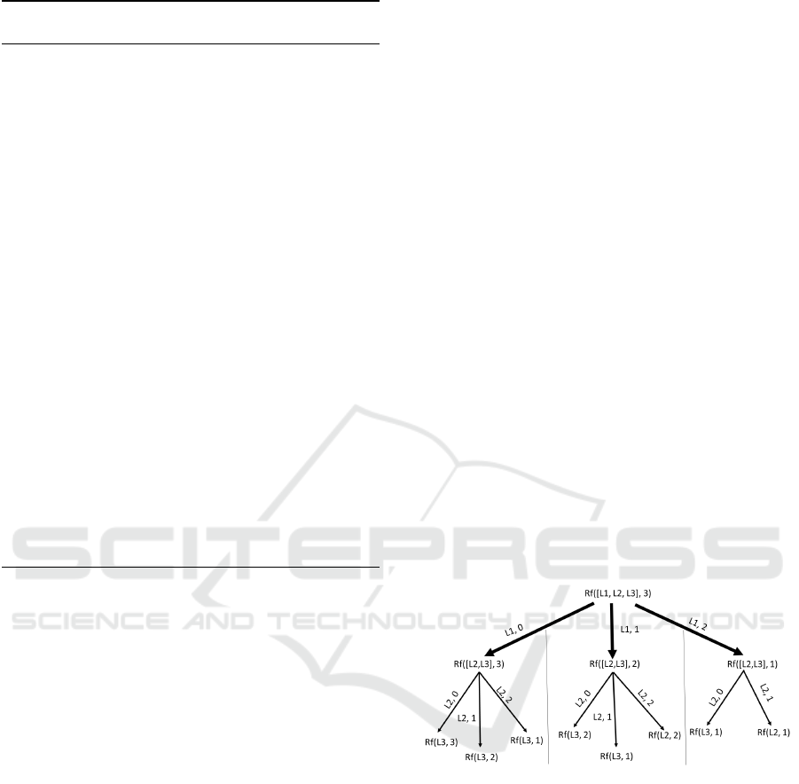
Figure 6: Combination possibilities of generating a 3-edge

interlayer substructure.

Figure 6 shows an example of the combinatorial

possibilities applied by the Combine-MLN recursive

function, where the set of layers is [L1, L2, L3] and

the substructure size is 3. For example, one possibility

is to choose 2 edges from L1 and 1 edge from either

L2 or L3 (the rightmost subtree) or 1 edge from L1,

one edge from L2, and 1 edge from L3 (middle sub-

tree.) Also, this composition stage ensures that only

connected composed substructures are generated.

Figure 7 illustrates the working of Combine-MLN

on a 2-layer MLN. For each layer we show all the

2-edge substructures. When we apply the Combine-

MLN function on each Vertex id of the graph as

shown above, we ﬁnd all the substructures of size

MLN-Subdue: Substructure Discovery In Homogeneous Multilayer Networks

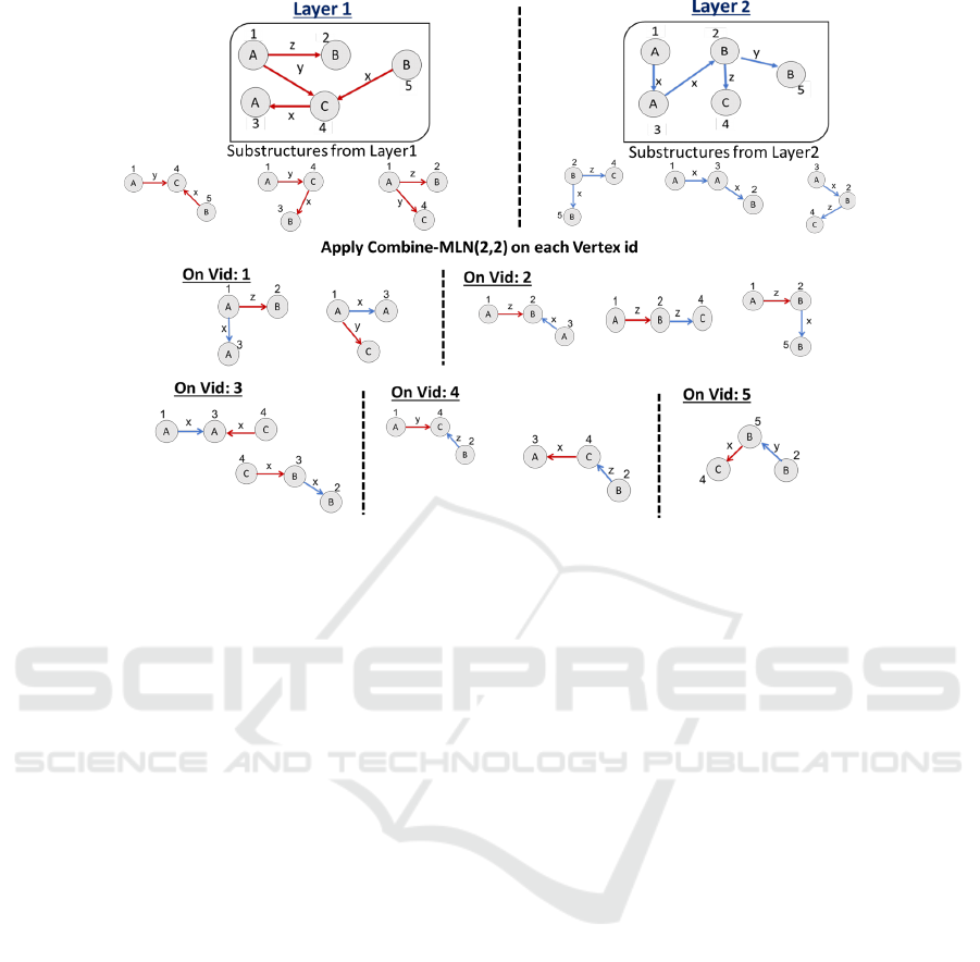
Figure 7: Generating composed interlayer substructures by combining intralayer substructures on shared vertex id.

2, which exist across layers. The parameters of

Combine-MLN function here is (2,2), which means

there are 2 layers and the required size of the sub-

structure is 2.

Duplicate Elimination: The previous step leads to

the generation of duplicate instances (e.g., from ﬁg-

ure 6, the center branch would be generated while

expanding on each of the three layers, L1, L2, and

L3.) As the composed substructures are cast into the

canonical form, duplicates are identiﬁed and removed

(Line 9).

Frequency Counting: Exact isomorphs are used

to detect identical substructures, as two isomorphic

substructures have the same relative ordering of the

vertex IDs and have same vertex and edge labels.

Canonical instances follow the lexicographic order-

ing, hence it is easy to generate k-edge canonical sub-

structures using the relative ordering of unique vertex

ID in the order of their appearance in the canonical

instance. All the instances are grouped based on their

canonical form and their frequency is counted (Line

12).

Application of Metric: To restrict the future expan-

sion to high quality substructures, a metric – either

MDL or frequency – is used to determine the impor-

tance of a particular substructure (Line 14). The beam

parameter (user speciﬁed with a default) is used as

a heuristic to ensure only the top beam substructures

based on the metric score will be passed on to the next

iteration, thereby restricting the expansion of less im-

portant substructures (Line 15).

Using the proposed algorithm, top substructures

of size k+1 that exist within and across layers in the

iteration are generated. Algorithm 1 is applied it-

eratively to ﬁnd substructures of the desired size.

6 MAP/REDUCE

IMPLEMENTATION

The different components of the proposed Algorithm

1 (layer-wise substructure expansion and duplicate

elimination followed by composition, and duplicate

elimination again in each iteration) have been imple-

mented using an iterative two-chained Map/Reduce

architecture. In the ﬁrst Map/Reduce job, the map-

per performs the expansion of substructures and du-

plicate elimination in each layer, and the reducer per-

forms the composition to generate substructures that

span layers and removes the duplicates from the com-

posed substructures. In the second job, the mapper

converts all substructure instances into canonical iso-

morphic instances to count frequency and emits iso-

morphs as key. The reducer applies the metric and

outputs the top-beam substructures (intralayer and

spanning layers) to be used as candidates for expan-

sion in the next iteration. Figure 8 shows the overall

workﬂow of substructure discovery in a HoMLN us-

ing the Map/Reduce framework.

Expansion by Mapper 1: Substructure instances

KDIR 2024 - 16th International Conference on Knowledge Discovery and Information Retrieval

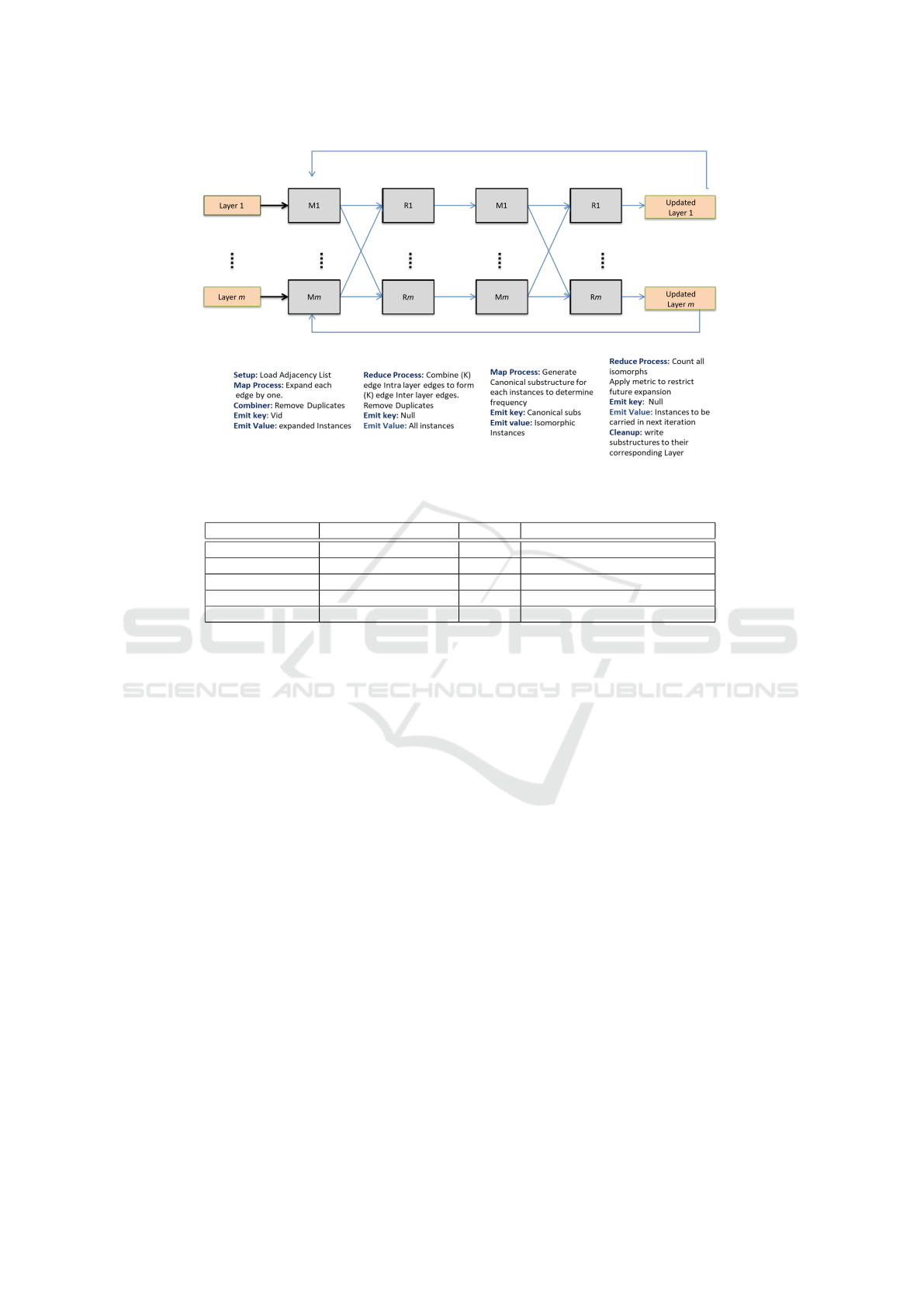
Figure 8: Map/Reduce workﬂow of MLN-Subdue (including composition).

Table 1: Dataset description.

Purpose Dataset #Nodes #Edges

Correctness Synthetic (SUBGEN) 10K 20K

Correctness Synthetic (SUBGEN) 100K 800K

Scalability LiveJournal 3.9M 34.8M

Scalability Orkut 3.87M 114.8M

Varying Density Synthetic (SUBGEN) 2K 1M, 1.9M, 2.9M, 3.9M

with their respective layer number are read as mapper

input, one at a time. The adjacency list for the layer is

loaded using the setup function. For the k

iteration,

the input is a k-edge canonical instance. Each instance

is expanded by one edge at a time using the adjacency

list. The mapper emits the vertex ID as key, and ex-

panded instances as values. As the expansion process

is unconstrained, duplicates are generated, which are

removed using a combiner. In this version, since each

layer is processed by a mapper (even as multiple map

tasks based on the block size), all duplicates can be

eliminated by the combiner.

Composition in Reducer 1: Each reducer receives

a list of expanded substructure instances as values,

grouped on the vertex ID as the key. The recur-

sive function (Combine-MLN) is used to combine all

(k + 1)-edge substructures from the mapper outputs

to generate (k + 1)-edge spanning substructures using

edges from multiple layers. All substructures, both

intralayer and spanning layers, are then emitted to the

next Map/Reduce job as input to generate canonical

substructures to determine graph isomorphism. The

key is null, and the value is the substructure instance.

Identifying Isomorphs in Mapper 2: Creating

canonical substructures from instances requires a

hash table to identify the relative positioning of each

vertex. The mapper receives all the substructure in-

stances as input, and canonical substructure is gener-

ated for every instance. The mapper emits the canoni-

cal substructure as the key and the corresponding sub-

structure instance as the value.

Ranking and Emitting top-beam Instances in

Reducer 2: The reducer receives substructure in-

stances across mappers grouped on canonical sub-

structure. The beam value is used to rank the best

beam substructures in a hash map. This is done by

calculating the MDL value for each canonical sub-

structure, and storing the top beam substructures with

the highest MDL values, emitting only their respec-

tive instances in order to restrict future expansion to

high-ranking substructures in the next iteration. The

reducer emits the (k + 1)-edge substructure instances

and layer IDs as the values in the k

iteration, which

are then fed into Mapper 1 of the next iteration as in-

put.

7 EXPERIMENTAL ANALYSIS

Experimental Setup: All experiments have been per-

formed using Java with Hadoop on Comet cluster

at SDSC (San Diego Supercomputer Center). The

MLN-Subdue: Substructure Discovery In Homogeneous Multilayer Networks

Comet cluster has 1944 nodes and each node has 24

cores (built on two 12-core Intel Xeon E5 2.5 GHz

processors) with 128 GB memory, and 320GB SSD

for local scratch space.

Dataset Description: Experiments were done on sev-

eral real-world and synthetic datasets (as shown in

Table 1) of varying sizes to establish the correctness,

speedup, and scalability of the approach. Subgen

, an

artiﬁcial graph generator was used to generate syn-

thetic graphs as it allows the embedding of substruc-

tures with user-deﬁned frequency in a larger single

graph. To generate HoMLN datasets from each base

single graph, edges were randomly distributed across

multiple layers among the same set of nodes.

Empirical Correctness: For a given HoMLN with

multiple layers, the ground truth is generated by ﬁrst

aggregating the MLN into a single graph by taking

the union of edges (Boolean OR) and then executing

SUBDUE(Ketkar et al., 2005). Both the proposed al-

gorithm and SUBDUE for different HoMLNs gener-

ated the same set of substructures with correct fre-

quency, thus establishing the correctness of the ap-

proach empirically.

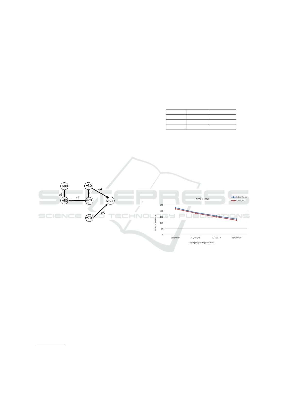
Figure 9: Example 5-edge Embedded Substructure.

However, SUBDUE being a main memory ap-

proach failed to execute on large graphs with more

than 100K vertices & 800K edges. So, to verify the

correctness on large graphs, synthetic graphs were

generated having substructures embedded with a user-

deﬁned frequency, the goal being to ﬁnd the same sub-

structures with the same frequency. A 5-edge embed-

ded substructure, shown in ﬁgure 9, was embedded

with a frequency of 1000 in a graph of size 100K

vertices & 800K edges. The exact substructure was

found with the same frequency (of 1000) using the

proposed algorithm, which empirically validates the

correctness of the proposed algorithm for this dataset.

Several such experiments were conducted with

different embedded graph sizes and frequencies.

Effect of Layer Generation Schemes: This set of

experiments is performed using the synthetic dataset

of size 400K vertices & 1.2 million edges with em-

bedded substructures. Two partitioning schemes were

https://ailab.wsu.edu/subdue/

used: random and edge-based, to verify the correct-

ness of the algorithm and its effect on response time.

Random scheme partitions a graph into l layers by

distributing edges randomly. Nodes are same in all

l layers. Edge-based partitioning, on the other hand,

creates layers containing all edges having the same

edge label. Multiple edge labels can be in a layer in

edge-based partitioning.

Table 2: Edge distribution for different layer generation

schemes.

Layers Random Edge-Based

Layer 1 399903 351360

Layer 2 399730 478441

Layer 3 400637 370469

Table 2 shows the edge distributions for both parti-

tioning schemes. Notice that the distribution remains

even for random partitioning, but becomes skewed for

edge-based as there can be edge labels with higher

frequency going into a single layer, making it uneven.

Figure 10 shows the total time taken by both of the

partitioning schemes. There is no substantial differ-

ence in the total response time as it more or less re-

mains the same. So, the numbers are drilled-down

into and the Map and Reduce times are inspected to

understand them clearly.

Figure 10: Total response time for partitioning schemes.

As seen in Figure 11, the total map time for edge-

based partitioning is signiﬁcantly higher as compared

to the total map time for random partitioning. The

reason being, as the edge distribution is skewed, some

mappers end up processing more data for edge-based

partitioning, contributing to more computation time.

On the other hand, total time taken by the reducers

does not change as the data processed by each re-

ducer remains the same, because all the substructures

in the reducer are grouped based on their vertex IDs

and edge labels have no effect on them.

The same embedded substructures were found for

both partitioning schemes, indicating that the algo-

rithm is not affected by the connectivity of the graph.

Scalability of Approach: Without altering the graph

size, an increase in the number of processors is typi-

KDIR 2024 - 16th International Conference on Knowledge Discovery and Information Retrieval

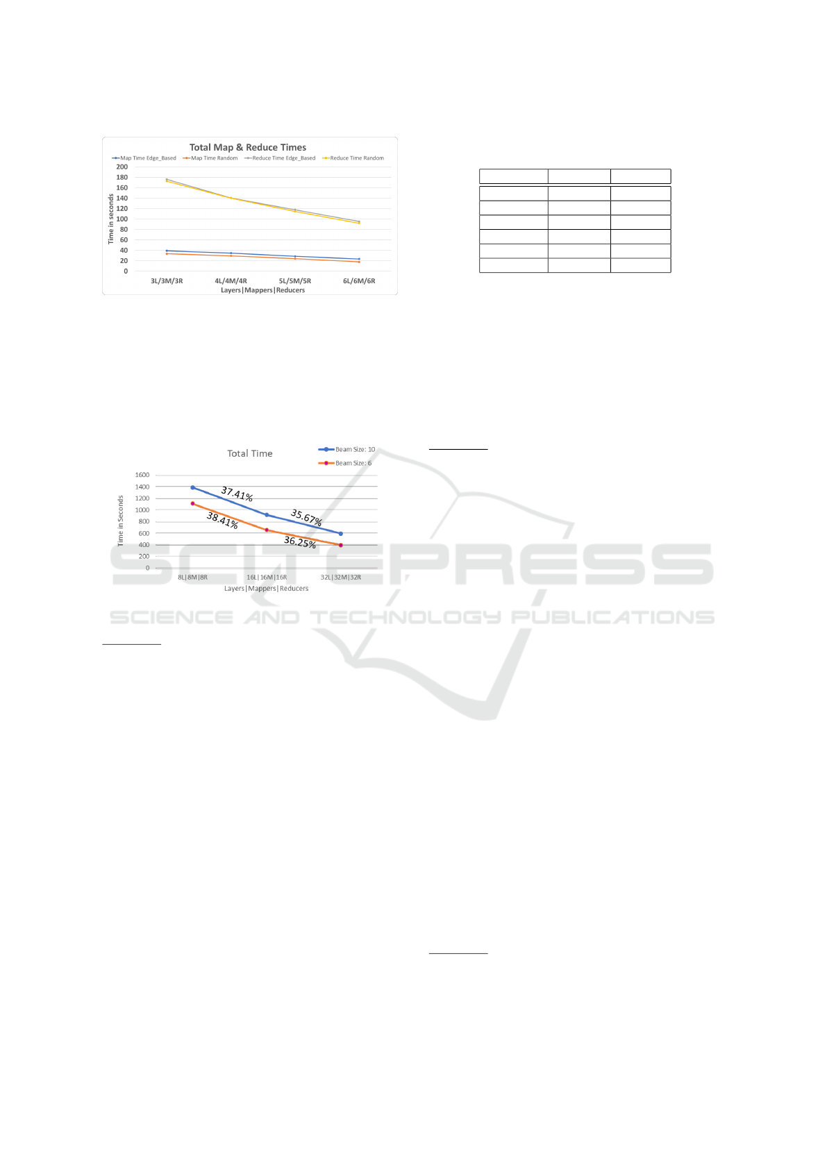
Figure 11: Map & Reduce times using multiple partitioning

schemes.

cally beneﬁcial for mining. So, this set of experiments

was performed on LiveJournal (Leskovec and Krevl,

2014a) and Orkut (Leskovec and Krevl, 2014b) data

to determine the speedup and effectiveness of the al-

gorithm as the number of processors was increased.

This has been showcased using 3 scenarios:

Figure 12: Speedup achieved on LiveJournal data.

Scenario 1: Same number of mapper and reducer

nodes as layers: For this scenario, all the layers are

processed in parallel with the same number of map-

per and reducer nodes. Results in Figure 12 show

a speedup of over 35% for the LiveJournal dataset

when the number of layers, mappers, & reducers are

increased from 8 to 16, and again from 16 to 32. As

the same dataset is partitioned into more layers and

processed by greater number of processors, it leads to

smaller partitions and less computation in each pro-

cessor. This reduction in computation cost contributes

to the speedup achieved. Moreover, as the number of

layers and reducers are doubled, the data received by

each reducer node gets halved, but the mining cost

in the 1st reduce job also increases, as the height of

the tree grows with the increase in number of layers

(as there are composed substructures that span more

layers and the number of combinations for the recur-

sive procedure Compose-MLN increases), leading to

a higher number of possible interlayer combinations.

Figure 12 also shows that the total time taken

when beam size is set to 10 is more as compared to

beam size 6. This is because as the beam size in-

Table 3: Number of substructures generated in each itera-

tion with beam 10 and 6 for the LiveJournal data.

Iterations Beam 10 Beam 6

1 2836928 2836928

2 3929240 3172184

3 4593864 3628496

4 5249968 3849008

5 5346152 4004984

6 5716984 4128496

creases, the number of substructures carried forward

in each iteration increases (illustrated in Table 3), re-

sulting in more data being processed by each proces-

sor.

Orkut and LiveJournal datasets were used for

the next two scenarios with 32 layers (Figures 13a,

13b.) The purpose is to understand the impor-

tance of mappers vs. reducers with respect to the

work/computation done during the algorithm.

Scenario 2: Changing only the number of reducer

nodes: In this scenario, the number of mapper nodes

is ﬁxed at 32, and the number of reducer nodes is var-

ied to see the effect of reducers on response time.

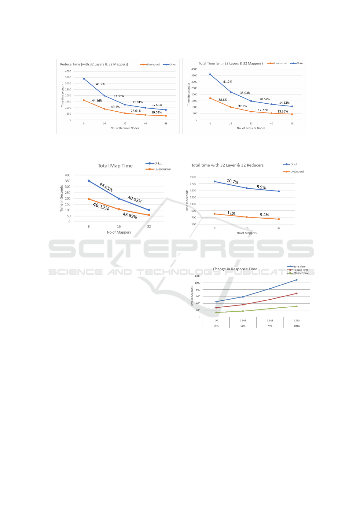
Figure 13a initially shows a high percentage of

speedup for both LiveJournal and Orkut in the re-

duce phase when the number of reducer nodes is in-

creased from 8 to 16 to 32. But after that, the speedup

starts to plateau, with the percentage improvement re-

ducing signiﬁcantly when going from 32 to 40 and

then to 48 nodes. So, merely adding more reducer

nodes beyond a certain number does not keep improv-

ing speedup, as the overhead (e.g., reducer setup &

cleanup) increases. Orkut takes more absolute time

than LiveJournal, as it has more than 3 times the num-

ber of edges for a similar number of vertices, leading

to more expansion and combination possibilities. In

contrast to the reduce time, total time is shown in

Figure 13b. This speedup is similar to the reduce

time (except in absolute values) indicating that all the

speedup comes from the reducers. This matches the

work done in the reducers as explained in Section 6

and validates the need for more reducers. Remem-

ber, composition is happening in the reducer of job 1

and counting all isomorphs and metric computation is

happening in the reducer of job 2.

Scenario 2 clearly indicates that the mappers take

less time overall as compared to the reducers. Hence,

distributing reduce computation among more re-

ducers has a signiﬁcant effect on the speedup

which is exempliﬁed in scenario 3 below.

Scenario 3: Changing only the number of mapper

nodes: Here, the number of reducer nodes is ﬁxed

at 32, and the number of mapper nodes is varied to

inspect the effect of mappers on response time.

MLN-Subdue: Substructure Discovery In Homogeneous Multilayer Networks

(a) Effect on Reduce Phase Time. (b) Effect on Overall Map/Reduce Time.

Figure 13: Speedup comparison by varying only the number of reducer nodes.

(a) Effect on Map Phase Time. (b) Effect on Overall Map/Reduce Time.

Figure 14: Speedup comparison on varying only the number of mapper nodes.

In Figure 14a, signiﬁcant speedup is seen in the

map time as the number of mapper nodes is increased

from 8 to 16 to 32. But the total time shown in Fig-

ure 14b is distinctly different from the one we see in

Figure 13b. Total time speedup has reduced signif-

icantly due to much smaller portion of the computa-

tion being distributed. This, again, clearly indicates

that there is not much computation in the mappers

to effectively distribute them to improve the over-

all Map/Reduce performance. In both jobs in the

chain, the reducers are doing heavy lifting in this ar-

chitecture. From Scenarios 2 and 3, it can be inferred

that for this algorithm, prioritizing an increase in the

number of reducers over mappers is more beneﬁcial,

as the reduce phase has a greater effect on total exe-

cution time.

Effect of Graph Density: Connectivity of graphs

also inﬂuences the performance of substructure dis-

covery due to large number of substructures gener-

ated during expansion. We categorize graphs as dense

to sparse, where the number of vertices is ﬁxed but

the number of edges vary along the spectrum ranging

from a completely connected graph to a very sparsely

connected graph. This experiment was performed on

a graph with 2K vertices, but varying densities from

Figure 15: Effect of graph density on response time.

25% (1M edges) to 100% (3.9M edges) on 4 layers

using 4 mapper nodes and 4 reducer nodes to see the

effect of connectivity of graphs on response time.

The results in Figure 15 show that with dense

graphs, where each vertex is connected to more ver-

tices on average, the computation cost increases as

there are more expansions which leads to more map

time and more combinations of intralayer edges in the

reducer contributing to more reduce time. This fur-

ther conﬁrms that more time is spent in the reducer in

this algorithm as compared to the mapper.

KDIR 2024 - 16th International Conference on Knowledge Discovery and Information Retrieval

8 CONCLUSIONS

This paper proposes a scalable substructure discov-

ery algorithm for HoMLNs using the decoupling-

based strategy. A generic Map/Reduce algorithm

was introduced for the parallel processing of lay-

ers and then composing the results, again, using a

Map/Reduce framework. The basic components of

substructure discovery - substructure expansion, com-

bining substructures from each layer to generate sub-

structures spanning layers (composition function),

duplicate elimination, and counting isomorphic sub-

structures - were incorporated into the Map/Reduce

framework. Empirical correctness was established.

Extensive experimental analysis was performed on di-

verse synthetic and real-world graph datasets.

ACKNOWLEDGMENTS

This work was supported by NSF awards #1955798

and #1916084.

REFERENCES

Berenstein, A., Magarinos, M. P., Chernomoretz, A., and

Aguero, F. (2016). A multilayer network approach

for guiding drug repositioning in neglected diseases.

PLOS.

Boccaletti, S., Bianconi, G., Criado, R., del Genio, C.,

omez-Garde

nes, J., Romance, M., Sendi

na-Nadal,

I., Wang, Z., and Zanin, M. (2014). The structure and

dynamics of multilayer networks. Physics Reports.

Boden, B., G

unnemann, S., Hoffmann, H., and Seidl, T.

(2012). Mining coherent subgraphs in multi-layer

graphs with edge labels. In Proceedings of the 18th

ACM SIGKDD International Conference on Knowl-

edge Discovery and Data Mining, KDD ’12, pages

1258–1266. ACM.

Bringmann, B. and Nijssen, S. (2008). What is frequent in

a single graph? In Paciﬁc-Asia Conf. on Knowl. Disc.

and Data Mining (PAKDD), pages 858–863. Springer.

Cook, D. J. and Holder, L. B. (1993). Substructure dis-

covery using minimum description length and back-

ground knowledge. Journal of Artiﬁcial Intelligence

Research, 1:231–255.

Das, S. and Chakravarthy, S. (2015). Partition and con-

quer: Map/reduce way of substructure discovery. In

International Conference on Big Data Analytics and

Knowledge Discovery, pages 365–378. Springer.

Das, S. and Chakravarthy, S. (2018). Duplicate reduction in

graph mining: Approaches, analysis, and evaluation.

IEEE Trans. Knowl. Data Eng., 30(8):1454–1466.

De Domenico, M., Sol

e-Ribalta, A., G

omez, S., and Are-

nas, A. (2014). Navigability of interconnected net-

works under random failures. Proc. of Ntl. Acad. of

Sciences.

Domenico, M. D., Nicosia, V., Arenas, A., and Latora, V.

(2014). Layer aggregation and reducibility of multi-

layer interconnected networks. CoRR, abs/1405.0425.

Elseidy, M., Abdelhamid, E., Skiadopoulos, S., and Kalnis,

P. (2014). Grami: Frequent subgraph and pattern min-

ing in a single large graph. Proceedings of the VLDB

Endowment, 7(7):517–528.

Ketkar, N. S., Holder, L. B., and Cook, D. J. (2005). Sub-

due: Compression-based frequent pattern discovery in

graph data. In Proceedings of the 1st Int. Workshop on

open source data mining: frequent pattern mining im-

plementations, pages 71–76.

Kivel

a, M., Arenas, A., Barthelemy, M., Gleeson, J. P.,

Moreno, Y., and Porter, M. A. (2013). Multilayer net-

works. CoRR, abs/1309.7233.

Leskovec, J. and Krevl, A. (2014a). LiveJournal - SNAP

Datasets: Stanford large network dataset collection.

http://snap.stanford.edu/data/com-LiveJournal.html.

Leskovec, J. and Krevl, A. (2014b). Orkut - SNAP Datasets:

Stanford large network dataset collection. http://snap.

stanford.edu/data/com-Orkut.html.

Liu, G. and Wong, L. (2008). Effective pruning techniques

for mining quasi-cliques. In Joint European confer-

ence on machine learning and knowledge discovery

in databases, pages 33–49. Springer.

Padmanabhan, S. and Chakravarthy, S. (2009). Hdb-

subdue: A scalable approach to graph mining. In

International Conference on Data Warehousing and

Knowledge Discovery, pages 325–338. Springer.

Pavel, H. R., Roy, A., Santra, A., and Chakravarthy, S.

(2023). Closeness centrality detection in homoge-

neous multilayer networks. In Proceedings of the 15th

International Joint Conference on Knowledge Discov-

ery, Knowledge Engineering and Knowledge Manage-

ment, IC3K 2023, KDIR.

Rao, R. B. and Lu, S. C. (1992). Learning engineering mod-

els with the minimum description length principle. In

AAAI, pages 717–722.

Santra, A., Bhowmick, S., and Chakravarthy, S. (2017a).

Efﬁcient community re-creation in multilayer net-

works using boolean operations. In International Con-

ference on Computational Science, ICCS 2017, 12-14

June 2017, Zurich, Switzerland, pages 58–67.

Santra, A., Bhowmick, S., and Chakravarthy, S. (2017b).

Hubify: Efﬁcient estimation of central entities across

multiplex layer compositions. In IEEE International

Conference on Data Mining Workshops.

Santra, A., Komar, K., Bhowmick, S., and Chakravarthy, S.

(2022). From base data to knowledge discovery – a

life cycle approach – using multilayer networks. Data

& Knowledge Engineering, page 102058.

Wang, W., Wang, C., Zhu, Y., Shi, B., Pei, J., Yan, X.,

and Han, J. (2005). Graphminer: a structural pattern-

mining system for large disk-based graph databases

and its applications. In Proceedings of ACM SIGMOD

2005, pages 879–881.

Yang, S., Yan, X., Zong, B., and Khan, A. (2012). Towards

effective partition management for large graphs. In

SIGMOD Conference, pages 517–528.

MLN-Subdue: Substructure Discovery In Homogeneous Multilayer Networks