Ensemble Learning Based Models and Deep Learning Model for

Credit Prediction, Case Study: Taiwan, China

Mingyuan Han

College of Alameda, 555 Ralph Appezzato, Memorial Pkwy, Alameda, CA 94501, U.S.A.

Keywords: Credit Prediction, Data Imbalance Processing, Machine Learning Model.

Abstract: As time progresses, credit prediction has become increasingly critical for banks and financial institutions. It

serves to optimize fund allocation and mitigate the risk of non-performing loans, thereby contributing to the

stability of the financial system. This study specifically delves into the credit market of Taiwan. Given the

inherent incompleteness of the dataset, preprocessing methods are imperative to address data imbalances.

Techniques such as oversampling, undersampling, and ensemble methods are employed for this purpose.Six

machine learning models are utilized to train the system for credit prediction: Logistic Regression (LR),

Decision Tree (DT), Random Forest (RF), Gradient Boosting Decision Trees (GBDT), Extreme Gradient

Boosting (XGBoost), and Deep Neural Network (DNN). To assess the performance of these models, cross-

validation and index evaluation methods are employed to ensure the robustness and reliability of the

findings.Upon comparison of five performance metrics across the six models, XGBoost emerges as the most

effective model for credit prediction in this context..

1 INTRODUCTION

After the coronavirus pandemic, much of the world's

businesses and individuals are experiencing financial

strain. In such circumstances, credit risk has escalated.

Simultaneously, the world is entering an era

characterized by the continuous development of

information technologies (Ma, 2017), offering

expanded opportunities for capital transactions.

Consequently, banks and other financing institutions

must ensure that borrowers do not default to safeguard

their investments (Zhang, 2018). Overall, credit

prediction is assuming heightened significance within

the financial system.

Over the past decade, banks have dedicated

substantial resources to developing internal risk

models to more effectively assess the financial risks

they encounter and allocate requisite economic

capital (Kwon, 2019; Wang, 2019). These endeavors

have garnered recognition and encouragement from

banking regulators. Notably, the Market Risk

Amendment (MRA) of the 1997 Basel Capital Accord

formally integrated banks' internal market risk models

into their regulatory capital computations (Zhang,

2020). Credit risk assessment plays a pivotal role in

https://orcid.org/0009-0005-0034-0068

appropriately assisting financial institutions in

crafting banking policies and business strategies.

In recent years, the proliferation of social lending

platforms has disrupted traditional credit risk

assessment services (Liu, 2020; Zhang, 2020; Chen,

2021). These platforms facilitate direct interaction

between lenders and borrowers, bypassing financial

intermediaries. They notably aid borrowers in

fundraising, enabling participation from lenders of

various numbers and sizes. However, the

inexperience of lenders and the absence or ambiguity

of information concerning borrowers' credit histories

may heighten the risk associated with social lending

platforms, underscoring the need for accurate credit

risk scoring.

To overcome these problems, the credit risk

assessment problem for financial operations is often

modeled as a binary problem based on debt repayment,

so appropriate machine learning techniques can be

utilized (Xu, 2021;Chen,2021).

Han, M.

Ensemble Learning Based Models and Deep Learning Model for Credit Prediction, Case Study: Taiwan, China.

DOI: 10.5220/0012910900004508

Paper published under CC license (CC BY-NC-ND 4.0)

In Proceedings of the 1st International Conference on Engineering Management, Information Technology and Intelligence (EMITI 2024), pages 115-121

ISBN: 978-989-758-713-9

115

2 METHODOLOGIES

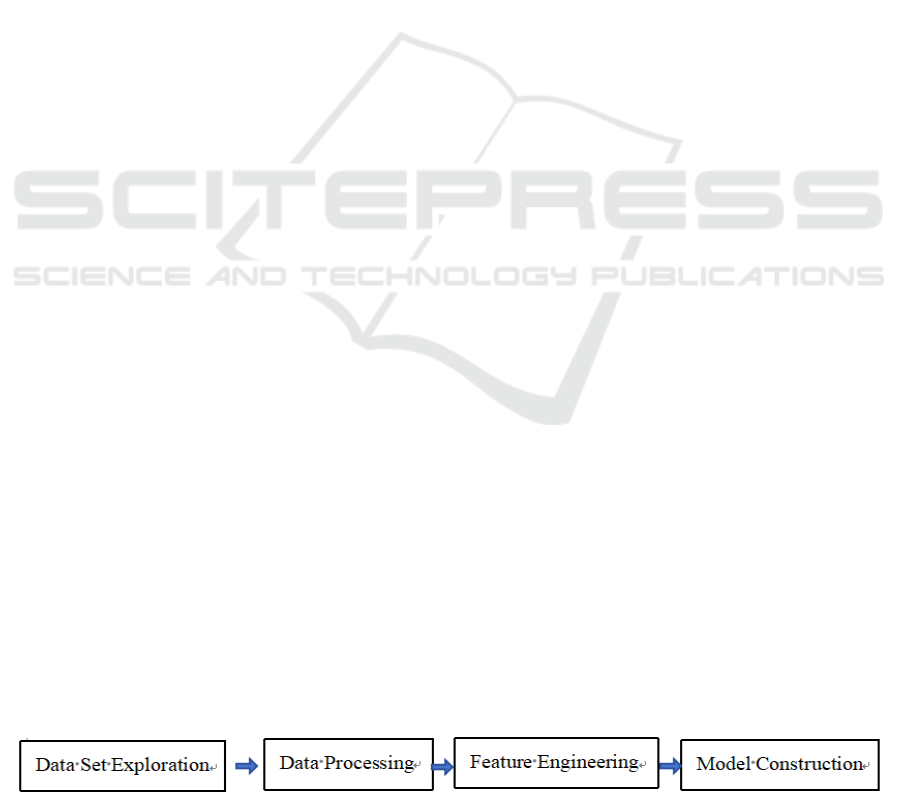
This research followed a structured approach

consisting of five main steps. Initially, a preliminary

analysis and visualization of the dataset were

conducted. The second step involved data

preprocessing to address any inconsistencies or

imbalances. Subsequently, the third step focused on

feature engineering to enhance the dataset's predictive

capabilities. The fourth step entailed selecting the

appropriate machine learning model for training. This

study employed six models: Logistic Regression (LR),

Decision Tree (DT), Random Forest (RF), Gradient

Boosting Decision Trees (GBDT), Extreme Gradient

Boosting (XGBoost), and Deep Neural Network

(DNN).

The final step encompassed a comparative

analysis of the model performance using five

evaluation indicators, leading to the identification of

the most suitable model. The workflow of the

research is illustrated in Figure 1 below.

2.1 Data Set Exploration

In the first step of this research was look at the first

few lines of the dataset to understand the basic

structure, features, and samples of the data. And then

use Python to find basic descriptive statistics of the

statistics, such as mean, median, standard difference,

etc., in order to get a preliminary understanding of the

distribution of the data. At the same time, it is also

necessary to draw some statistical charts and

correlation heat maps of data characteristics. The

specific content of chart analysis will be shown in the

Experimental Setup and Results of the fourth part of

the paper.

2.2 Data Processing

Taking the data collected in questionnaire survey as

an example, respondents often fill in some survey

questions with blanks. This can also simply explain

that data sets generally have certain problems of

missing and inauthentic. In order to avoid the impact

of numerical missing and data anomalies on the

efficiency and performance of machine learning, it is

necessary to preprocess the data set. In this study,

oversampling synthesis, oversampling and

undersampling were used to deal with data imbalance.

The data set consists of 30,000 observations. Use

70% as the training set and 30% as the test set after

the data preprocessing step.

2.3 Feature Engineering

Feature engineering is an important part of machine

learning. This includes the selection of feature values

and the labeling of features. In this research, the data

set has 24 eigenvalues, such as age, sex, education and

so on. Some of these features have little relevance to

credit forecasting research, so it is necessary to do

some feature selection in the research. The second is

the feature tag coding. Some feature types in the data

set represent high-dimensional information. Feature

screening can reduce the noise generated by low

correlation feature values in machine learning, so as

to improve research efficiency and accuracy. High

dimensional information needs to be reduced, which

is simply to use different numbers to represent

different features in the same feature type.

2.4 Model Selection and Construction

In this study, the feature types include both high-

dimensional information and continuous data such as

credit card consumption amount and repayment

amount. So the six machine learning models used in

the study also include linear model. In order to make

more comprehensive predictions of credit, the six

models used in this survey include linear models, tree

models (including three ensemble learning methods)

and deep learning models. Ensemble learning is a

machine learning model that combines multiple

learners. The performance and generalization ability

of the whole model can be improved by the prediction

of multiple learners. By incorporating multi-level

nonlinear learning, deep neural networks can

autonomously acquire intricate feature

representations. This model proves highly effective

for credit forecasting, particularly when considering

multiple criteria.

● Linear Regression

Linear regression is based on the basic assumption

that there is a linear relationship between input

features and output targets. This means that output

targets can be predicted by linear combinations of

Figure 1: Research Workflow(Photo/Picture credit :Original).

EMITI 2024 - International Conference on Engineering Management, Information Technology and Intelligence

116

input features. In this study, scikit-learn library was

used to complete the training of regression models

● Decision Tree

A Decision Tree is a supervised learning algorithm for

classification and regression problems. It divides the

data recursively to generate a tree structure, with each

leaf node representing a category or a value. Decision

trees are a non-parametric learning method that makes

no assumptions about the distribution of data and is

suitable for all types of data. The main advantage of

decision trees is that they are easy to understand and

interpret, but also easy to overfit.

●Random Forest

Random Forest is an ensemble learning method that

improves prediction performance by building

multiple decision trees and integrating them together.

In the process of building each tree, the random forest

will randomly sample the original data set with a

return to generate different training data to increase

the diversity of the model. Random forest performs

well in dealing with high-dimensional data, large-

scale data and high complexity problems, and does

not require too much tuning. It is a powerful machine

learning model that is widely used for tasks such as

classification, regression, and feature selection.

●Gradient Boosting Decision Tree

GBDT is a powerful machine learning algorithm

based on ensemble learning. Its integrated learner is

the same as RF, and it improves prediction

performance by training multiple decision trees in

serial. GBDT adopts a sequential training strategy, in

which each decision tree is trained according to the

residuals of the previous tree to gradually reduce the

residuals of the model. The task of each decision tree

is to learn the residual predicted by the previous tree

(the difference between the actual value and the

current model predicted value) in order to reduce the

error of the overall model. As a result, GBDT can

handle mixed data and is robust to missing values.

●XGBoost

XGBoost is a powerful gradient lift tree model, whose

operation steps include initializing the base model,

iteratively building a new decision tree to fit the

residuals of the previous round of models, and

gradually integrating multiple trees to improve

performance. By controlling tree complexity through

regularization techniques, XGBoost excels in

handling structured data, large data sets, and

challenging tasks, becoming one of the algorithms of

choice in machine learning competitions and real-

world applications.

●Deep Neural Network

Deep neural network is a flexible and powerful deep

learning model, whose operation steps include

defining the network structure, initializing the

parameters, calculating the model output through

forward propagation, updating the parameters

through backpropagation, and continuously

improving the model fitting ability through multiple

iterations of training. DNN is suitable for processing

high-dimensional, non-linear and large-scale data,

and is widely used in image recognition, natural

language processing and complex pattern recognition,

with powerful feature learning and representation

learning capabilities.

3 EXPERIMENTAL SETUP AND

RESULTS

3.1 Data Set Overview

This research uses the credit records of Taiwan as the

data set. The selected dataset contains a total of

30,000 observations with 24 feature types (shown in

Table 1).

Table 1: Description of feature types.

Feature abbreviation Feature data type data range

LIMIT

BAL Line of Credi

Discrete T

pe Ten Thousand-A Million

SEX Gende

Discrete T

pe 1,2

EDUCATION Schoolin

Discrete T

pe 0,1,2,3,4,5,6

MARRIAGE Marital Status Discrete T

pe 0,1,2,3

AGE A

e Discrete T

pe 21--79

PAY

0-PAY

6 Repa

ment Times Discrete T

pe -2--8

defaul

men

nex

month Default next month Discrete T

pe 0,1

Ensemble Learning Based Models and Deep Learning Model for Credit Prediction, Case Study: Taiwan, China

117

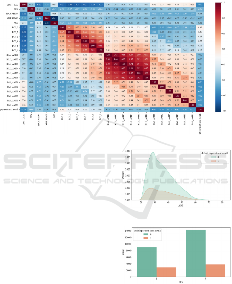
Figure 2: Attribute Correlation Matrix(Photo/Picture credit :Original).

This study also analyzes the relationship between

each characteristic and default which is presented by

Attribute Correlation Matrix (Figure 2).

Attribute Correlation Matrix is typically used to

describe the degree of association between different

attributes in a dataset. Specifically, the attribute

correlation matrix is a square matrix whose elements

represent the correlation coefficients between

different attributes in the data set. The correlation

coefficient measures the strength and direction of the

linear relationship between two variables. The figure

can also analyze whether default has a high

correlation with credit limit. The higher the credit

limit, the lower the probability of default. (Figure 2)

Additionally, the research encompasses

individual feature analyses, which are visually

represented through mapping. These analyses

visually elucidate the correlation between features

and default occurrences, aiding in the identification of

potential research focal points (Feature 3, Figure 4,

Figure 5, Figure 6). From the ensuing charts, four key

insights emerge: default probabilities are higher for

males compared to females; a higher educational

attainment correlates with a reduced default rate;

unmarried individuals exhibit a higher default

probability than their married counterparts; and

individuals in their 30s manifest the lowest default

rates.

Figure 3: The Relationship between Age and Default

(Photo/Picture credit: Original).

Figure 4: The Relationship between Gender and Default

(Photo/Picture credit: Original).

EMITI 2024 - International Conference on Engineering Management, Information Technology and Intelligence

118

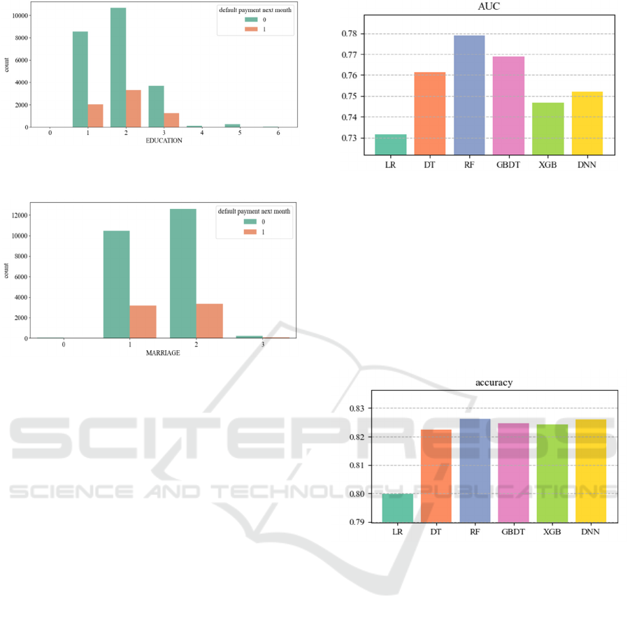
Figure 5: The Relationship between Education and

Default(Photo/Picture credit :Original).

Figure 6: The Relationship between Marriage and Default

(Picture credit: Original).

3.2 Experimental Settings

All models were implemented in Python 3.8.5

environment in this research. Then, this research had

used seven packages: Use pandas for data processing

and analysis. Numerical calculations were performed

using numpy. Use matplotlib.pyplot and seaborn for

visualization. Use the imblearn to handle class

imbalances. Tensorflow was used to build and train

deep learning models. Use the os for file and directory

operations. The experimental hardware was

configured with a 2.40GHz i7-13700H CPU, an

RTX4060GPU, and 16GRAM.

3.3 Model Evaluation

The AUC is the area under the ROC curve, which

describes the tradeoff between the true case rate and

the false positive case rate at different classification

thresholds. The closer the AUC value is to 1, the

better the model performance and better classification

ability. Of the six models in the figure 7, random

forest has the highest AUC value. Second is GBDT,

decision tree.

Figure 7: AUC Comparison Diagram (Photo/Picture credit:

Original).

Accuracy is the proportion of the number of

samples correctly predicted to the total number of

samples. Accuracy is an important metric in many

cases, but may not be comprehensive enough in cases

where categories are unbalanced. As can be seen from

the figure 8, except for linear regression, the other five

models have higher accuracy and smaller gap

between them. Among them, RF and DNN performed

best.

Figure 8: Accuracy Comparison Diagram (Photo/Picture

credit: Original).

Precision is the percentage of all samples that are

predicted to be positive cases that are actually positive

cases. Precision measures the accuracy of the model

in positive case predictions and is suitable for

situations where the focus is on reducing false

positives. In the figure 9, XGboost performs best. RF

and XGBT are similar. In the figure 9, DNN has the

best effect, followed by RF and DT.

The recall rate refers to the proportion of actual

positive cases that are correctly predicted as positive

cases by the model, also known as the true case rate.

The recall rate measures how well the model covers

positive examples and applies to situations where the

focus is on finding as many positive examples as

possible. As can be seen from the figure 10, DNN has

the highest recall rate. This was followed by DT, RF,

Ensemble Learning Based Models and Deep Learning Model for Credit Prediction, Case Study: Taiwan, China

119

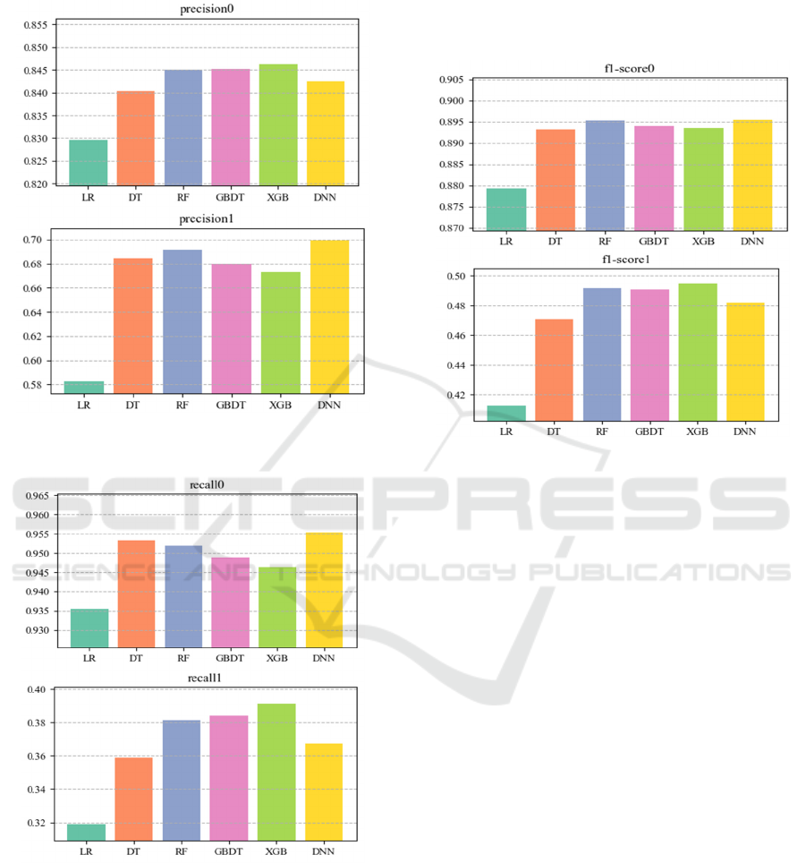
GBDT and XGboost. The other chart shows the

highest performance of XGBoost.

Figure 9: Precision Comparison Diagram (Photo/Picture

credit:Original).

Figure 10: Recall Comparison Diagram (Photo/Picture

credit: Original).

The F1 score serves as a harmonic average of

accuracy and recall, offering a balanced perspective

on their relationship. It proves particularly beneficial

in scenarios characterized by imbalanced data,

effectively weighing both accuracy and recall,

thereby enhancing model evaluation. In the final

performance metric, among the five models depicted

on the left, all but LR exhibit comparable

performance. Notably, XGBoost demonstrates

superior performance in the right image, with RF,

GBDT, and DNN following suit (see Figure 11).

Figure 11: F1-Score Comparison Diagram.

4 CONCLUSION

This study employs six machine learning models to

analyze and predict the Taiwan credit dataset,

encompassing linear models, tree models, and deep

neural network models. Specifically, these models

include Linear Regression, Decision Trees, Random

Forests, Gradient Boosting Decision Trees, Extreme

Gradient Boosting, and Deep Neural Networks.

Through a comprehensive comparison of

performance across five dimensions, it is evident that

GBDT and XGBoost models exhibit superior

performance, with Deep Neural Network ranking

third. Both GBDT and XGBoost are renowned

representatives of gradient boosting methods within

the realm of machine learning. By amalgamating

multiple weak learners, GBDT adeptly captures

nonlinear relationships, thereby ensuring high

prediction accuracy while also assessing feature

importance.

XGBoost, built upon the foundation of GBDT,

further enhances model efficiency through the

incorporation of regularization terms, parallel

computation, and automated handling of missing

feature values. These enhancements significantly

augment training and prediction efficiency while

bolstering the model's generalization capabilities.

EMITI 2024 - International Conference on Engineering Management, Information Technology and Intelligence

120

Both models offer compelling advantages such as

robust interpretation, the capacity to model intricate

data patterns, and overall robustness. However,

XGBoost's enhancements in speed, efficiency, and

regularization render it particularly favored in

practical applications.

Consequently, when confronted with diverse

problem domains, it is advisable to leverage GBDT

and XGBoost models due to their robust performance

and suitability for practical deployment.

REFERENCES

Chen, S., Liu, G., & Liao, S. , 2021. Credit risk assessment

using ensemble deep learning with interpretable

features. Expert Systems with Applications, 167,

114183.

Chen, X., Luo, Y., Guo, W., & Hu, X. , 2021. Credit risk

assessment using deep learning ensemble models with

credit scorecard. Knowledge-Based Systems, 223,

106983.

Kwon, O., & Kang, S. , 2019. Credit risk prediction using

ensemble deep learning. Expert Systems with

Applications, 134, 330-342.

Liu, Z., & Zheng, W. , 2020. Credit risk evaluation using

deep learning and ensemble learning. Applied Soft

Computing, 90, 106208.

Ma, Y., Liu, Y., Hu, X., & Zhang, H. , 2017. Credit risk

assessment with a deep ensemble-learning approach.

Expert Systems with Applications, 83, 19-28.

Wang, S., Ding, Y., Guo, W., & Hu, X. , 2019. Credit risk

assessment based on deep learning ensembles. Expert

Systems with Applications, 118, 178-190.

Xu, Y., Li, J., & Zhang, J. , 2021. Deep ensemble learning

for credit risk prediction. Applied Soft Computing, 107,

107458.

Zhang, Y., Ma, J., Zhou, L., & Liu, W. , 2018. Credit risk

assessment using ensemble learning: A systematic

literature review. Expert Systems with Applications, 114,

19-34.

Zhang, Y., Zheng, Y., & Liu, W. , 2020. A hybrid deep

learning model for credit risk assessment. Expert

Systems with Applications, 147, 113203.

Zhang, Y., Zheng, Y., & Liu, W. , 2020. A novel hybrid

credit scoring model based on deep learning and

ensemble learning. Knowledge-Based Systems, 197,

105975.

Ensemble Learning Based Models and Deep Learning Model for Credit Prediction, Case Study: Taiwan, China

121