Contrastive Learning and Abstract Concepts: The Case of

Natural Numbers

Daniel N. Nissani (Nissensohn)

Independent Research, Israel

Keywords: Contrastive Learning, Self-Supervised Learning, Learning Representations, Generalization, Counting,

Subitizing, Natural Numbers, Conservation Principles.

Abstract: Contrastive Learning (CL) has been successfully applied to classification and other downstream tasks related

to concrete concepts, such as objects contained in the ImageNet dataset. No attempts seem to have been made

so far in applying this promising scheme to more abstract entities. A prominent example of these could be the

concept of (discrete) Quantity. CL can be frequently interpreted as a self-supervised scheme guided by some

profound and ubiquitous conservation principle (e.g. conservation of identity in object classification tasks).

In this introductory work we apply a suitable conservation principle to the semi-abstract concept of natural

numbers by which discrete quantities can be estimated or predicted. We experimentally show, by means of a

toy problem, that contrastive learning can be trained to count at a glance with high accuracy both at human as

well as at super-human ranges. We compare this with the results of a trained-to-count at a glance supervised

learning (SL) neural network scheme of similar architecture. We show that both schemes exhibit similar good

performance on baseline experiments, where the distributions of the training and testing stages are equal.

Importantly, we demonstrate that in some generalization scenarios, where training and testing distributions

differ, CL boasts more robust and much better error performance.

1 INTRODUCTION AND

RELATED WORK

Contrastive Learning (CL) is a self supervised

scheme which has attracted much attention in recent

years. In the visual modality realm it maps a visual

input (e.g. objects to be classified) to linearly

separable representations which achieve

classification accuracy rates competitive with those

of supervised learning (SL) networks of similar

architecture (Chen et al., 2020) in challenging

datasets such as ImageNet (Deng et al., 2009).

In spite of its impressive success in the space of

concrete concepts (Chen et al., 2020), neither CL nor

its variants (Grill et al., 2020; He et al., 2020; Chen &

He, 2020) have been apparently applied so far to the

learning and prediction of abstract or semi-abstract

entities. In a recent work (Nissani (Nissensohn),

2023) has shown that CL can (unlike SL) build

“hyper-separable” representations which are useful

not only to predict an object identity but also to

indicate the existence (or absence) of selected

attributes of interest of this object; this might be seen

as a first modest step away from the concrete and

towards the abstract. Another prominent example of

the learning, ‘grounding’, or in-depth ‘understanding’

of such an abstract entity could be that of the concept

of natural numbers (equivalently, discrete quantities).

This work is a preliminary and introductory step

forward in this direction.

CL exploits, in the concrete visual modality, a

profound principle of conservation: that distinct

views of an object preserve the identity of said object.

To create such distinct views suitable transformations

should (and generally can) be designed (Tian et al.,

2020). Analog principles of conservation have been

applied in physics (e.g. conservation of energy, of

momentum, etc. under suitable reference frames

transformations) with extraordinary success during

the last two centuries.

To apply a relevant and useful transformation to

our (discrete) quantity prediction challenge within a

CL scheme we can imagine the following thought

experiment: that we have objects which we wish to

count at a glance (that is “count without counting”,

see ahead), that these objects lay at the bottom of a

closed box with transparent cover. Shaking the box,

Nissani (Nissensohn), D.

Contrastive Learning and Abstract Concepts: The Case of Natural Numbers.

DOI: 10.5220/0012917500003837

Paper published under CC license (CC BY-NC-ND 4.0)

In Proceedings of the 16th International Joint Conference on Computational Intelligence (IJCCI 2024), pages 523-530

ISBN: 978-989-758-721-4; ISSN: 2184-3236

523

our transformation, will randomly change the layout

of the objects inside the box, but the total number of

objects on the box floor will be conserved (since the

box is closed, etc.).

Our CL optimization goal l(i, j) will then consist

of minimizing the normalized distance (Wang &

Isola, 2020) between the neural network so called

projection (i.e. last) layer (Chen et al., 2020)

representations z

and z

of the pre- and post-shaking

views (‘positive samples’ in the CL jargon) while

simultaneously maximizing the distances between

these representations and the representations of other

samples randomly gathered in a mini-batch (‘negative

samples’). Formally, our goal will then be (see Chen

et al., 2020 for details):

𝑙

(

𝑖,𝑗

)

= (1)

−

𝑠𝑖𝑚𝑧



,𝑧





𝜏

+ log ( 1







exp (

𝑠𝑖𝑚

(

𝑧



,𝑧



)

𝜏

)

𝐿 = (2)





∑

[𝑙

(

2𝑘 − 1,2𝑘

)

+ 𝑙

(

2𝑘,2𝑘 − 1

)

]





where sim(. , .) is the normalized inner product (i.e.

the cosine similarity), τ is a system temperature, N is

the mini-batch size, 1



is a binary indicator function

which vanishes when k = i and equals 1 otherwise,

and L is the overall loss, i.e. l(i, j) summed over all

samples in the mini-batch. At the end of the

optimization process we freeze the neural network

learned parameters, fetch an interior layer and define

its output to be our linearly separable representation

vectors. These are then fed into a (usually supervised,

single layer) linear classifier.

We humans are able to estimate at a glance, with

high precision and with no explicit enumeration, a

relatively small (up to between 4 to 7) number of

objects in view (Trick & Pylyshyn, 1994). This

capability, for which the special term ‘subitizing’ was

coined (Kaufman et al., 1949) has motivated in recent

years a few groups of neural networks practitioners

(Chattopadhyay et al, 2017; Acharya et al., 2018) to

explore the application of supervised learning (SL)

schemes to a similar challenge.

We are not aware of any similar work on natural

numbers under the umbrella of CL, nor of the

application of CL schemes to other non-tangible

concepts.

As a preliminary introduction to these ideas we

implement a toy problem and corresponding datasets

by means of which CL and SL networks of similar

architecture are trained to subitize and predict the

quantity of identical objects present in an image. We

compare the error performance of these two schemes

at both a ‘baseline’ regime, where training and testing

data originate from identical distributions, as well as

at various generalization regimes, where training and

testing data distributions differ. CL is trained by a

more profound, potentially ‘grounding’, criterion

than SL, a criterion that is intimately related to the

concept of Quantity itself. We thus may well suspect

that it will exhibit error performance better than that

of SL, at least in some of the forementioned

generalization regimes.

The main contributions of this introductory work

are:

a. We demonstrate through the example of the

Quantity (equivalently, Natural Numbers)

non-tangible concept, that CL can learn

abstract concepts whenever transformations

which conserve their defining properties can

be identified and implemented.

b. We show that both CL and SL can learn to

subitize, both at human range (order of 10

objects) and super-human range (order of

100). Moreover, that the error performance of

CL and SL are similarly good under the

forementioned baseline regime scenarios.

c. We show that CL exhibits significant error

performance superiority over SL under certain

generalization regime scenarios, possibly

corroborating, as suspected, the more

profound and grounded nature of learning by

means of a conservation principle (relative to

SL learning which consists of merely forcing

representations to adjust to arbitrary labels).

In Section 2 the toy problem and test setup which

we introductorily employ to demonstrate these ideas

are presented. Section 3 details our simulation results,

and Section 4 provides concluding remarks and

outlines potential future lines of research.

2 EXPERIMENTAL SETUP

We implement a toy problem to conduct experiments,

demonstrate our ideas and probe into our CL

superiority conjecture. We generate (practically

infinite) sequences of random synthetic images of

dimension d x d pixels, with d = 22 or 28. Each image

contains a number of identical white objects laid out

over a black background. For each experiment we

select a training dataset distribution {O, S, R} and a

testing dataset distribution {O’, S’, R’} so we

designate an experiment by the composite triplet

{O/O’, S/S’, R/R’}.

NCTA 2024 - 16th International Conference on Neural Computation Theory and Applications

524

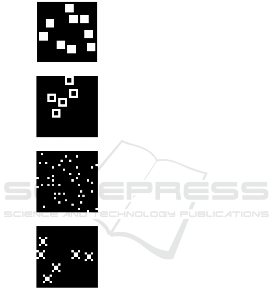
Figure 1: Synthetic image samples. Each image of d x d

pixels (d = 28 in this Figure) contains a random layout of a

random number of objects of an identical shape. Shapes are

either (from top to bottom) Full squares (denoted F in the

text), Void squares (V), Dots (D) and Crosses (C); we may

either preset the objects shape for all images within the

dataset with the same selected shape, or randomly pick for

each image a fixed shape amongst F/V/C which we denote

by X (for miXed, not shown in Figure). The shapes

definition is thus an element of {F, V, C, D, X}.

Baseline experiments consist of triplets where O

= O’, S = S’ and R = R’; otherwise they are

Generalization experiments wherein the training and

testing distributions differ.

O is the maximal number of objects in an image

and took in our experiments the values 10 (to emulate

human range), 60 or 80 (for super-human); the

number of objects in an image is uniformly randomly

selected within a subset of [1, O].

S defines the shape of all objects within an image

and, for the sake of some shape diversity, can take the

values F, V, C, D or X (see Figure 1 for details).

R can take the values A (for All), E (for Evens) or

O (for Odds) where A means that the number of

objects in an image can be any in the range [1, O]

while E or O restricts this number to the subset of

even or odd values respectively.

A typical experiment may consist of {O/O’, S/S’,

R/R’} = {80/80, D/D, A/A} which means identical

training and testing distribution (i.e. a Baseline

experiment) with between 1 to 80 objects in each

image, each object of Dot shape, and no Evens nor

Odds only restriction.

The objects are randomly laid out within the

image. We do not allow objects to occlude nor touch

each other. Each sample image is generated along

with its label which describes the number of objects

in that sample.

We train a simple fully connected multi layer

neural network by CL with architecture [d

400 400

100] where the last layer, of dimension 100, is the (so

called) projection layer (Chen et al., 2020) and the

penultimate layer, of dimension 400 is our

representation layer.

We use for SL an identical architecture, except for

the last layer which for SL contains a softmax

activation function of dimension O. Note that we

could instead have chosen to implement a regression

(e.g. linear) scheme for SL. We opted for the former

since it supports a more ‘apples to apples’

comparative study.

It is not so simple to physically emulate the

“shaking of our box” (of our thought experiment

above) in order to create a new image sample with the

same number of objects within it but with a different

random objects layout. Instead, we opt for a

surrogate: we take the label attached to each image

(which describes the number of objects in that image)

and use it to generate another (random layout) image

with this specified number of objects. This may seem

at first glance a cheating perversion by which we

convert our CL (unsupervised learning) scheme into

a supervised learning one (since we are now using

labels for our ‘transformation’). After some reflection

Contrastive Learning and Abstract Concepts: The Case of Natural Numbers

525

however, it should be easy to conclude that this is

immaterial to our purpose. The same results we are

going to show can be exactly replicated by a true

physical shaking of our box.

Training of CL or SL proceeded for a number of

samples until no further visible convergence progress

is observed in the Loss goal (Eqns. (1) and (2) above

for CL) or in the training Mean Squared Error goal

(for SL). Once training is halted we freeze the CL (or

SL) parameters, and train a single layer supervised

linear classifier (Oord et al., 2018) with the CL (or

SL) network representations generated by the testing

dataset distribution. After this linear classifier is

trained, we evaluate error performance with samples

generated by means of this same selected test dataset

distribution (as mentioned above our datasets are

practically infinite so we are not, by no means and as

properly prohibited, re-using samples for both

training and testing).

We set the CL hidden layers neural units

activation to ReLU and the last layer units to tanh. CL

temperature (τ of Equation 1) was set to 1, and batch

size (N of Equation 2) was set to 10

. We used ADAM

(Kingma & Ba, 2015) gradient descent with fixed

learning rate η = 10

-3

. The number of training samples

ranged from 1.8 x 10

(equivalent to e.g. 30 MNIST

epochs) to 3.6 x 10

depending on the running

experiment.

SL units were here again set to ReLU for hidden

layers but to softmax activation for the last layer. We

used ADAM with fixed learning rate η = 5 x 10

-4

for

the initial stage followed by plain gradient descent

with learning rate typically descending from 10

-5

-7

. We found this protocol necessary to achieve our

best error performance, possibly testifying the

navigation within a deep narrow valley (Martens,

2010). The number of SL training samples ranged

from 4.2 x 10

to 10.8 x 10

Finally, the linear classifier was trained by ADAM

followed by plain SGD, with similar optimization

protocol as that of SL above and number of samples

typically ranging from 2.4 x 10

to 28.8 x 10

Across all three above schemes ADAM parameters

were set to β

= 0.9, β

= 0.999 and e = 10

-8

To facilitate replication of our results a simulation

package will be provided by the author upon request.

3 SUBITIZING EXPERIMENTAL

RESULTS

In this Section we will be comparing CL vs. SL

subitizing error performance. To probe whether our

forementioned conjecture, which states that CL will

boast superior performance w.r.t. SL in at least some

of the Generalization scenarios (where training and

test distributions differ) we define a set of appropriate

experiments. We also provide baseline results (where

training and testing distributions are identical) for

reference.

Generalization here can be applied along the

shape dimension, or the quantity dimension, or both

at a time (which we do not pursue herein). For

convenience we list below the experiments

(generalized item bold and underlined; please refer to

Section 2 for triplets legend):

• Shape Dimension (human range; train with

miXed images, test with Dots):

o Baseline: {O/O’, S/S’, R/R’} = {10/10,

X/X, A/A}

o Generalization: {O/O’, S/S’, R/R’} =

{10/10, X/D, A/A}

• Quantity Dimension, Range extension (super

human range; train with up to 60 objects, test

with up to 80):

o Baseline: {O/O’, S/S’, R/R’} = {60/60,

D/D, A/A}

o Generalization: {O/O’, S/S’, R/R’} =

{60/80, D/D, A/A}

• Quantity Dimension, within Range (super

human range; train with up to 80 objects, Even

values only, test with up to 80, All values):

o Baseline: {O/O’, S/S’, R/R’} = {80/80,

D/D, E/E}

o Generalization: {O/O’, S/S’, R/R’} =

{80/80, D/D, E/A}

• Quantity Dimension, within Range (super

human range; train with up to 80 objects, Even

values only, test with up to 80, Odd values

only):

o Baseline: {O/O’, S/S’, R/R’} = {80/80,

D/D, E/E}

o Generalization: {O/O’, S/S’, R/R’} =

{80/80, D/D, E/O}

3.1 Shape Dimension (Human Range;

Train with Mixed Images, Test with

Dots)

We report Pr

CL, B

{error} = 0.042 and Pr

SL, B

{error} =

0.007 for Baseline test (denoted by B in super-script),

i.e. {O/O’, S/S’, R/R’} = {10/10, X/X, A/A}, for CL

and SL respectively.

That SL yields better performance than CL under

baseline tests with similar networks architecture is no

surprise: it was noticed in prior works, see e.g. (Chen

et al. 2020) where in order to achieve similar error

NCTA 2024 - 16th International Conference on Neural Computation Theory and Applications

526

performance a deeper and wider architecture (on CL

network relative to SL) was required.

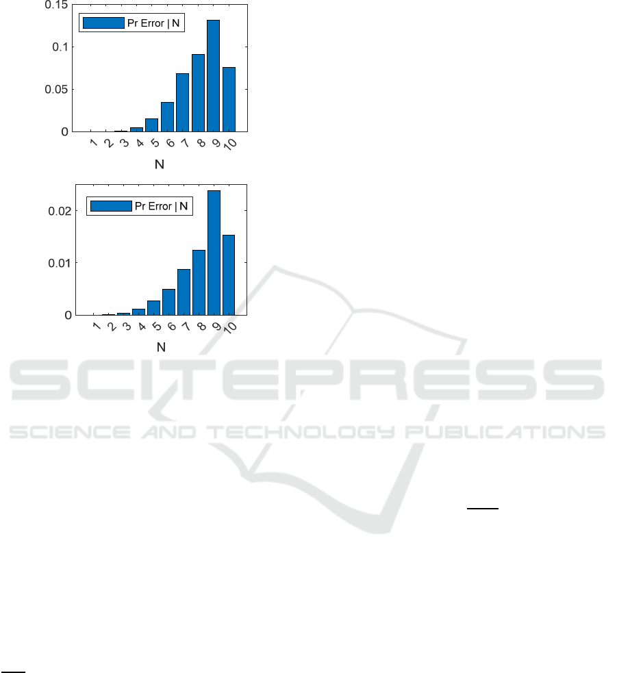
Figure 2: Shape Baseline test, 10 Objects, train with miXed,

test with miXed. Conditional probability of Error given

Ground Truth for CL (top) and SL (bottom).

Interestingly, errors are not uniformly distributed

across ground truth values at both CL and SL (see

Figure 2): as might be intuitively expected error rate

steadily increases from small to large ground truth

values (with 10 a possible curious exception; this may

be an artifact of our setup: since we set a hard limit of

10 through our softmax function, errors at this ground

truth value are contributed, unlike at other values, by

one side only). A qualitatively similar phenomenon

was observed in subitizing experiments conducted

with human subjects (Kaufman et al., 1949). We did

not observe however a similar trend with our

experiments at super human range.

We next turn to the corresponding Shape

Generalization test, i.e. {O/O’, S/S’, R/R’} = {10/10,

X/D, A/A} where training is conducted with miXed

images (which, as described above, contain either F

or V or C objects but do not contain Dots) but testing

is done with Dots images. Error probability

significantly degrades, with similar degradation at CL

and SL: Pr

CL, G

{error} = 0.31 and Pr

SL, G

{error} = 0.30

(superscript G here denotes Generalization).

More important perhaps however in a quantity

estimation task than this gross error measure is the

conditional distribution of Distances (conditioned on

error events), where Distance = |Ground Truth value

– Predicted value|: in practical situations to predict a

value of 8 instead of a ground truth value 9 is

forgivable while to predict a 1 in the same case is not.

This more suitable metric can be observed in

Figure 3: we notice that in spite the significant

forementioned Pr{error} degradation, the distribution

of Distance in both CL and SL is remarkably

concentrated in the very low values, with Pr

{Distance > 1 | error} = 0.036 and Pr

SL G

{Distance

> 1 | error} = 0.041, again pretty similar to each other.

To summarize, in this Shape Generalization

experiment CL and SL perform similarly; they both

degrade significantly in terms of Pr{error}, but their

more tolerant (and perhaps relevant) Pr{Distance > 1

| error} metric is still pretty good.

We have provided this Figure to contrast vs. next

experiments, as we will immediately see.

3.2 Quantity Dimension, Range

Extension (Super Human Range;

Train up to 60 Objects, Test with

up to 80)

Here we report Pr

CL, B

{error} = 0.029 and Pr

SL,

{error} = 0.004 for the Baseline test, i.e. {O/O’,

S/S’, R/R’} = {60/60, D/D, A/A}, for CL and SL

respectively. Since the Distance distribution metrics

is apparently of more significant relevance in

subitizing tasks we also report for the Baseline test

CL B

{Distance > 1 | error} = 0.035 and Pr

{Distance > 1 | error} = 0.002.

The corresponding Quantity Generalization test is

{O/O’, S/S’, R/R’} = {60/80, D/D, A/A} where

training is conducted with up to 60 Dots images and

testing is done with up to 80 Dots images. Again, as

in the Shape Generalization experiment, error

probability significantly degrades, with similar

degradation at CL and SL: Pr

CL, G

{error} = 0.24 and

SL, G

{error} = 0.23.

Conditional Distance distributions of CL and SL,

however, are totally different. Please refer to Figure

4. While CL Distance distribution is concentrated in

the very low values (as in our earlier experiments) and

CL G

{Distance > 1 | error} = 0.12, SL distribution

practically explodes with Pr

SL G

{Distance > 1 | error}

= 0.80.

Briefly summarizing so far, in shape

generalization experiments (Subsection 3.1 above)

both CL and SL behave similarly: this is reasonable

since it is not shape what CL learns in depth and thus

they should not differ much from each other, just as

in baseline tests.

Contrastive Learning and Abstract Concepts: The Case of Natural Numbers

527

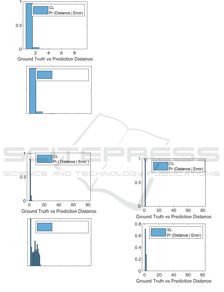
Figure 3: Shape Generalization, train with miXed, test with

Dots. Conditional probability distribution of Ground Truth

vs. Predicted Distance for CL (top) and SL (bottom).

Figure 4: Quantity Generalization, train with up to 60, test

with up to 80 Dots images. Conditional Distance

distribution for CL (top) and SL (bottom). CL exhibits a

modest degradation w.r.t. baseline test while SL collapses.

In contrast, in quantity generalization scenarios,

CL and SL respond extremely differently and CL

significantly outperforms SL. This can be attributed

in our view to the profoundness to which CL learns

the abstract concept of “numberness” by means of the

contrastive learning conservation principle,

compared to the merely forced mapping of input

images to arbitrary labels in SL. The concept of

Numbers seems to become ‘grounded’ in CL but not

so in SL.

3.3 Quantity Dimension, Within Range

(Super Human Range; Train with

up to 80 Objects, Even Values

Only, Test with up to 80, All

Values)

Next we report Pr

CL, B

{error} = 0.019 and Pr

SL,

{error} = 0.0004 as well as Pr

CL B

{Distance > 2 |

error} = Pr

SL B

{Distance > 2 | error} = 0 for the

Baseline test of this experiment, i.e. {O/O’, S/S’,

R/R’} = {80/80, D/D, E/E}, for CL and SL

respectively. Notice that conditional Distance

distribution results here are reported w.r.t. a threshold

valued 2 (rather than 1 as before) since Odds “do not

exist” in this Baseline scenario.

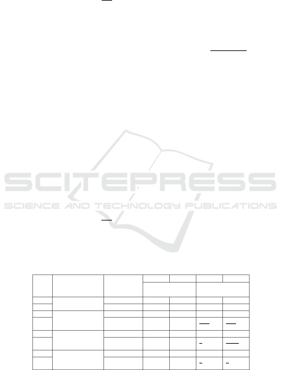
Figure 5: Quantity Generalization, train with Evens only,

test with All, both up to 80 Dots images. Distance

distribution for CL (top) and SL (bottom). CL exhibits no

degradation w.r.t. baseline test while SL once again

collapses.

2468

Ground Truth vs Prediction Distance

0.5

Pr (Distance | Error)

0 20406080

Ground Truth vs Prediction Distance

0.05

0.1

0.15

0.2

Pr (Distance | Error)

NCTA 2024 - 16th International Conference on Neural Computation Theory and Applications

528

The corresponding Quantity Generalization test is

{O/O’, S/S’, R/R’} = {80/80, D/D, E/A} where

training is conducted with even quantities (i.e. 2, 4.

6…80) of up to 80 Dots images, and testing is done

with all quantities (i.e. 1, 2, 3….80) of up to, again,

80 Dots images. SL degrades its error probability

w.r.t. baseline here, while CL this time exhibits even

better performance than its own baseline: Pr

{error} = 0.045 and Pr

CL G

{error} = 0.00003.

Evaluating again with our conditional Distance

distribution metrics (please refer to Figure 5), CL

significantly outperforms SL here too with Pr

{Distance > 1 | error} = 0 and Pr

SL G

{Distance > 1 |

error} = 0.285, supporting once again our motivating

conjecture.

3.4 Quantity Dimension, Within Range

(Super Human Range; Train with

up to 80 Objects, Even Values

Only, Test with up to 80, Odd

Values Only)

Our baseline setup here is identical to that of the last

experiment, i.e. {O/O’, S/S’, R/R’} = {80/80, D/D,

E/E}, for CL and SL respectively, and so are our

results. The conditional Distance distributions results

here (for both baseline and generalization tests) are

once again reported w.r.t. a threshold valued 2 (rather

than 1) for the same reason as in Subsection 3.3

above.

The corresponding Quantity Generalization test is

{O/O’, S/S’, R/R’} = {80/80, D/D, E/O} where

training is conducted with even quantities (i.e. 2, 4.

6…) of up to 80 Dots images and testing is done with

odd quantities (i.e. 1, 3, 5…79) of up to 79 Dots

images. Both CL and SL exhibit good error

probability with Pr

CL G

{error} = 0.026 and Pr

{error} = 0.026 and both show excellent Distance

conditionals with Pr

CL G

{Distance > 2 | error} = Pr

{Distance > 2 | error} = 0.

It appears that once CL and SL learn the Evens

the discriminative resolution of the resulting

representations is good enough to predict the Odds

with good error performance, For the SL scheme

however, this holds only provided that the Evens are

omitted from the testing dataset, so that they do not

‘confuse’ the SL network as apparently occurred in

our previous Subsection 3.3 experiment.

Table 1 provides a concise summary of our results

above.

4 DISCUSSION AND TOPICS

FOR FUTURE RESEARCH

We have provided preliminary demonstrative

evidence, through our selected example of quantity

estimation at a glance, that contrastive learning

methods can deal not only with concrete, tangible

concepts. Our choice however of natural numbers is

not casual. When

dealing with concrete objects it is

not difficult to identify transformation sets, with

random properties, which efficiently span the

distribution of a dataset; examples include crop and

color distortion for ImageNet (Chen et al., 2020) and

elastic distortion (Simard et al, 2003) for EMNIST

(Nissani (Nissensohn), 2023). This is possibly not the

case for abstract concepts in general, and identifying

viable abstract sets and their corresponding spanning

random transformations is a research challenge. It

would be of interest to see other such concepts to

follow-on our current very first step.

Table 1: Experiments results summary. T denotes a Threshold, valued 1 for all tests, except 5, 7 and 8 for which T = 2 (see

text). Most informative results are bolded/underlined.

Test

EXPERIMENT TEST CL SL CL SL

Pr{error} Pr{Distance > T |

error}

1 Shape, train

miXed test Dots

Baseline 0.042 0.007 0 0

2 Generalized 0.31 0.30 0.036 0.041

3 Qty, Range

extension, train 60

test 80 ob

ects

Baseline 0.029 0.004 0.035 0.002

4 Generalized 0.24 0.23 0.12 0.80

5 Qty, within

Range, train

Evens test All

Baseline 0.019 0.0004 0 0

6 Generalized 0.00003 0.045 0 0.285

7 Qty, within

Range, train

Evens test Odds

Baseline 0.019 0.0004 0 0

8 Generalized 0.026 0.026 0 0

Contrastive Learning and Abstract Concepts: The Case of Natural Numbers

529

We find it quite remarkable that both CL and SL

exhibit such impressive subitizing error performance

in baseline test scenarios even at super-human ranges.

We did not inquire into the existence of a practical

upper bound to this range nor, more generally, into

the error performance as function of the dataset range,

which of course should be of interest.

The results shown indicate that CL and SL perform

quite similar to each other in shape generalization

tests, both with significant error probability

degradation but with robust figures w.r.t. conditional

distance distribution. This might be expected since

the natural numbers conservation principle guiding

CL should not grant it any advantage when dealing

with varying shapes.

In contrast, CL alone maintains this robustness in

quantity generalization tests as well, and in particular

in range extension tests, where the scheme is asked to

estimate at a glance a quantity bigger than what it was

ever exposed to. This seems to support our motivating

conjecture that stated that CL, because it is guided by

the principle of conservation of natural numbers

should obtain, after training, a more deep and

grounded sense of ‘numberness’. And this would then

be the second case in a row at which CL seems to

show a fundamental superiority over SL in generating

information rich representations (the first being the

forementioned capability of detection of objects

attributes (Nissani (Nissensohn), 2023)).

In this introductory work we have devised and

employed a toy problem to demonstrate our ideas

because it has better control of test bench variables

and parameters. It should be of course important to

evaluate whether similar results can be achieved in

more realistic scenarios which may include clutter,

occlusion, composite scenes with different classes of

real-life objects, etc. Several datasets for such

purpose are already available (Acharya et al., 2019).

REFERENCES

Acharya, M., Kafle, K., Kanan, C., ‘TallyQA: Answering

Complex Counting Questions’, AAAI 2019

Chattopadhyay, P., Vedantarn, R., Selvaraju, R.R., Batra,

D., Parikh, D., ‘Counting Everyday Objects in

Everyday Scenes’, CVPR 2017

Chen, T., Kornblith, S., Norouzi, M., Hinton, G., ‘A Simple

Framework for Contrastive Learning of Visual

Representations’, PMLR 2020

Chen, X., He, K., ‘Exploring Simple Siamese

Representation Learning’, arXiv 2011.10566, 2020

Deng, J., Dong, W., Socher, R., Li, L., Li, K., Fei-Fei, L.,

‘ImageNet: A Large-Scale Hierarchical Image

Database’, CVPR 2009

Grill, J., Strub, F., Altche, F., Tallec, C., Richemond, P.H.,

Buchatskaya, E., Doersch, E., Pires, B.A., Guo, Z.D.,

Azar, M.G., Piot, B., Kavukcuoglu, K., Munos, R.,

Valko, M., ‘Bootstrap Your Own Latent. A New

Approach to Self-Supervised Learning’, arXiv

2006.07733, 2020

He, K., Fan, H., Wu, Y., Xie, S., Girshick, R., ‘Momentum

Contrast for Unsupervised Visual Representation

Learning’, arXiv 1911.05722v3

Kaufman, E.L., Lord, M.W., Reese, T.W., Volkmann, J.,

‘The Discrimination of Visual Number’, The American

Journal of Psychology, 1949, pp. 498-525

Kingma, D.P., Ba, J.L., ‘ADAM: A Method for Stochastic

Optimization’, ICLR 2015

Martens, J., ‘Deep learning via Hessian-free optimization’,

Proceedings of the 27

International Conference on

Machine Learning, 2010

Nissani (Nissensohn), D.N., ‘Contrastive Learning and the

Emergence of Attribute Associations’, ICANN 2023

Oord, A.v.d., Li, Y., Vinyals, O., ‘Representation Learning

with Contrastive Predictive Coding’, arXiv

1807.03748, 2018

Simard, P.Y., Steinkraus, D., Platt, J.C., ‘Best Practices for

Convolutional Neural Networks Applied to Visual

Document Analysis’, ICDAR 2003

Tian, Y., Sun, C., Poole, B., Krishnan, D., Schmid, C.,

Isola, P., ‘What Makes for Good Views for Contrastive

Learning?’, NIPS 2020

Trick, L.M., Pylyshyn, Z.W., ‘Why are Small and Large

Numbers Enumerated Differently? A Limited Capacity

Pre-attentive Stage in Vision”, Psychological Review,

1994

Wang T., Isola, P., ‘Understanding Contrastive

Representation Learning through Alignment and

Uniformity on the Hypersphere’, ICML 2020

NCTA 2024 - 16th International Conference on Neural Computation Theory and Applications

530