Comparison of Lateral Controllers for Autonomous Vehicles Based on

Passenger Comfort Optimization

Akos Mark Bokor

1 a

, Adam Szabo

2 b

, Szilard Aradi

2 c

and Laszlo Palkovics

1,3 d

Systems and Control Laboratory, HUN-REN Institute for Computer Science and Control (SZTAKI),

Kende utca 13-17., H-1111 Budapest, Hungary

Department of Control for Transportation and Vehicle Systems, Faculty of Transportation Engineering and Vehicle

Engineering, Budapest University of Technology and Economics, M

uegyetem rkp. 3., H-1111 Budapest, Hungary

echenyi Istv

an University, Egyetem t

er 1., H-9026 Gy

or, Hungary

Keywords:

Autonomous Vehicles, Genetic Algorithm, Model-Based Control, Optimization.

Abstract:

This paper focuses on the design of lateral controllers for autonomous vehicles. To enhance passenger comfort

while concurrently maintaining minimal deviation from the desired trajectory, the developed controllers are

tuned by a Genetic Algorithm, whose cost function is following the ISO 2631 Standard. Three model-based

controllers, a Linear Quadratic Regulator, a Linear Quadratic Servo algorithm, and a Model Predictive Con-

troller have been compared in a simulation environment. The test case consists of a suburban road section,

where the vehicles must successfully traverse at different velocities while minimizing the lateral acceleration

and jerk affecting the passengers. To take into account the velocity-dependent dynamics of the system, the

controllers are based on a Linear Parameter-Varying model of the system. The results show that the devel-

oped controllers meet the speciﬁed requirements regarding the equivalent acceleration, Motion Sickness Dose

Value, and deviation from the desired trajectory.

1 INTRODUCTION

Research into vehicle lateral control has been an on-

going endeavor since the 1950s and remains a criti-

cal aspect of autonomous vehicle design in the face

of evolving technological needs and challenges. Al-

gorithms based on geometric principles such as Pure

Pursuit (Samuel et al., 2016) and Stanley controllers

(AbdElmoniem et al., 2020) have been successfully

used in several cases. Yet, these controllers of-

ten fail at handling more complex, dynamic driving

tasks. Subsequently, model-based solutions were in-

troduced. Initially, these were based on linear mod-

els, but they have progressively shifted towards more

complex nonlinear model-based strategies (Menhour

et al., 2012). Each evolution offers distinct advan-

tages and confronts speciﬁc limitations, particularly

the challenge of dealing with variable system param-

eters that complicate the development of ﬁxed-gain

controllers.

https://orcid.org/0009-0005-4845-9923

https://orcid.org/0000-0003-1633-5588

https://orcid.org/0000-0001-6811-2584

https://orcid.org/0000-0001-5872-7008

Over the years, several key considerations have

shaped the design of lateral controllers. These in-

clude robust stability, computational capacity, and

precise reference signal tracking (G

asp

ar et al., 2016;

Tagne et al., 2015). However, integrating passenger

comfort into control system designs has become es-

sential as the industry achieves SAE Level 5 auton-

omy. This integration is crucial for enhancing mar-

ketability and providing a human-like driving expe-

rience (Cascetta et al., 2022). In recent years, this

goal has been pursued through machine learning al-

gorithms. For example, (Zhang et al., 2018) presents

an approach that utilizes a deep reinforcement learn-

ing algorithm to replicate human-like car-following

behavior with higher accuracy and adaptability than

traditional models. This integration ensures a more

accurate imitation of human driving styles and con-

tinuously updates the models with new data, enhanc-

ing the system’s adaptability and reliability in diverse

driving scenarios (Zhu et al., 2018), which is essential

for guaranteeing user safety and building trust in au-

tonomous systems. This can be achieved through var-

ious approaches; for instance, (Poussot-Vassal et al.,

2011) emphasizes using gain scheduling techniques

Bokor, A., Szabo, A., Aradi, S. and Palkovics, L.

Comparison of Lateral Controllers for Autonomous Vehicles Based on Passenger Comfort Optimization.

DOI: 10.5220/0012923700003822

Paper published under CC license (CC BY-NC-ND 4.0)

In Proceedings of the 21st International Conference on Informatics in Control, Automation and Robotics (ICINCO 2024) - Volume 1, pages 46-54

ISBN: 978-989-758-717-7; ISSN: 2184-2809

to adjust control parameters, enhancing vehicle dy-

namic stability.

The method proposed in (Li et al., 2019) breaks

the vision-based lateral control system down into a

perception and a control module. While the algo-

rithm outperformed model-based algorithms, there

are no guarantees regarding their robustness and

stability. Hence, another approach is to combine

machine-learning-based solutions with more conven-

tional control systems. Such an example is presented

in (Mashadi et al., 2014), where a Genetic Algorithm

is utilized to optimize a PID controller.

Besides ensuring precise reference tracking, the

emphasis on optimizing passenger comfort is rapidly

increasing. However, improved precision comes at

the cost of higher lateral acceleration, which may neg-

atively impact passenger comfort.(Tagne et al., 2015;

Mesghali, 2021) Addressing the trade-off between

precision in tracking and passenger comfort is par-

ticularly acute at higher speeds, where sharper ma-

neuvers lead to greater lateral accelerations. To mit-

igate these effects, implementing a speed-dependent

controller design is crucial. Techniques such as Gain

Scheduling and Linear Parameter Varying (LPV) con-

trol offer viable solutions to adjust controller gains

based on vehicle speed (N

emeth and G

asp

ar, 2011;

Zin et al., 2008; T

oth, 2010), thus optimizing both

performance and comfort across varying driving con-

ditions.

1.1 Related Work

Numerous methodologies exist for the design of con-

trollers that prioritize passenger comfort as a funda-

mental criterion for optimization. One such technique

involves minimizing the Motion Sickness Dose Value

(MSDV). The MSDV, adhering to the ISO 2631-1

standards, provides a quantitative index of passen-

ger comfort by explicitly accounting for the effects

of motion on the human vestibular system. The al-

gorithm proposed in (Moreno-Gonzalez et al., 2022)

is engineered to mitigate motion-induced discomfort

among passengers by adeptly managing vehicle dy-

namics, including acceleration and jerk.

In addition to minimizing the MSDV, passenger

comfort considerations can also be integrated into the

controller design. In (Sever et al., 2021), a gain-

scheduled Linear Quadratic Regulator (LQR) con-

troller is employed for this purpose, incorporating

modiﬁcations to account for both vertical and hori-

zontal motion components. This consideration is crit-

ical, as passengers, no longer needing to focus on

driving, may engage in activities that heighten their

susceptibility to motion sickness. A more traditional

approach is presented in (Luciani et al., 2020), where

the controllers are tuned concerning vehicle dynam-

ics and passenger comfort. The proposed method

integrates these considerations through a specialized

Model Predictive Control (MPC) design, optimizing

standard metrics for vibration and motion sickness

within the broader context of vehicle control.

These papers demonstrate that incorporating pas-

senger comfort considerations into controller design

does not signiﬁcantly diminish the controllers’ path-

following capabilities. Instead, they produce substan-

tially better comfort outcomes than controllers de-

signed solely for path-following. However, there is

a notable gap in research comparing these optimized

controllers despite the potential for varying results

in both simulations and practical applications. This

highlights the importance of conducting more com-

parative analyses to understand their relative effec-

tiveness under similar comfort considerations.

1.2 Contributions

This paper presents three model-based lateral con-

trollers, which are tuned through an optimization al-

gorithm that incorporates a cost function consisting of

tracking accuracy and passenger comfort-related re-

quirements. The presented controllers are evaluated

and compared based on their performance with re-

spect to the equivalent acceleration, MSDV, and lat-

eral deviation.

The paper is organized as follows: Section 2

presents the Linear Parameter-Varying model describ-

ing the lateral vehicle dynamics. Section 3 and Sec-

tion 4 describe the implemented control algorithms

and the applied optimization algorithm. Section 5

deals with the simulation environment and test cases,

while Section 6 presents the evaluation of the results.

Section 7 shows some concluding remarks.

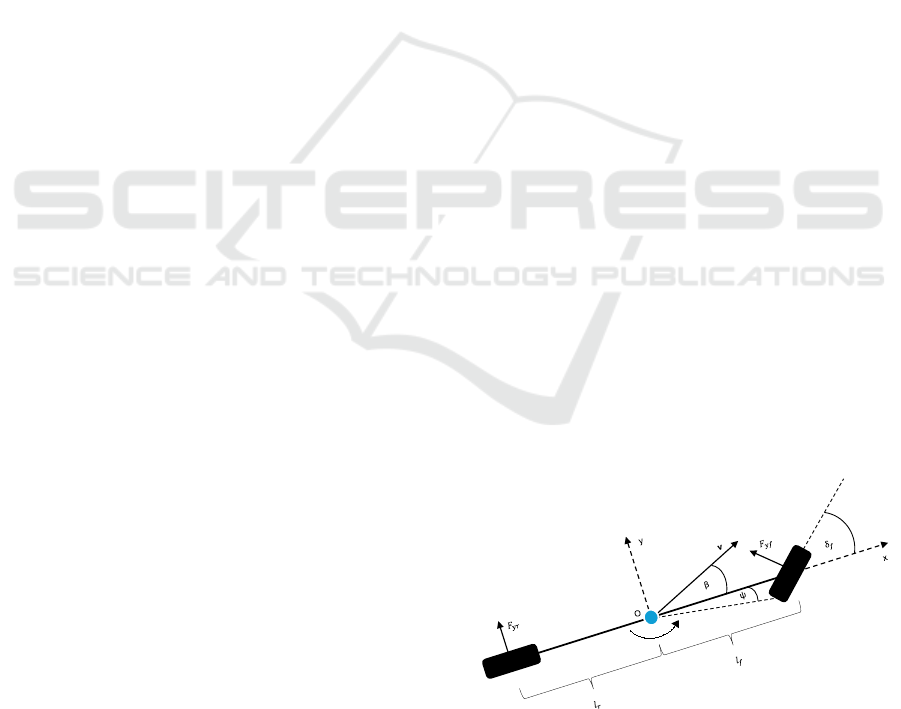
Figure 1: Lateral vehicle dynamics.

Comparison of Lateral Controllers for Autonomous Vehicles Based on Passenger Comfort Optimization

2 LATERAL VEHICLE MODEL

This paper uses a modiﬁed variant of the widely

known dynamic bicycle model, representing the ve-

hicle as a two-wheel-point system. Figure 1 shows

the lateral vehicle dynamics.

The equations of motion are derived as follows by

applying Newton’s second law and neglecting the im-

pact of road bank angle:

= F

y f

+ F

(1)

where a

is the inertial acceleration of the vehicle at

the center of gravity (c.g.) of the vehicle along the y-

axis, m is the mass of the vehicle, and F

y f

and F

are

the front and rear lateral tire forces, respectively.

The inertial acceleration of the vehicle consists of

two components: lateral acceleration and centripetal

acceleration. Hence, the lateral motion of the vehicle

can be written as follows:

m( ¨y +V

ψ) = F

y f

+ F

(2)

where ¨y is the lateral acceleration of the vehicle, V

the longitudinal velocity at the c.g., and

ψ is the yaw

rate.

The torque balance equation, which deﬁnes the

yaw dynamics of the vehicle, is written as follows:

ψ = ℓ

y f

− ℓ

(3)

where I

is the inertia of the vehicle along the z-axis,

ℓ

and ℓ

are the distances between the c.g. of the

vehicle and the front and rear tires, respectively.

Accounting for the interdependence between tire

forces and steering dynamics, the lateral tire forces

y f

and F

are calculated by determining the rela-

tionship between slip angle and lateral force. The slip

angle, which is the difference between the orientation

of the wheel and the wheel velocity vector, directly

inﬂuences the lateral forces.

Assuming a linear relationship between the tire

forces and the slip, the front and rear lateral tire forces

are deﬁned as follows:

y f

= 2C

(δ − θ

y f

) (4)

= 2C

(−θ

) (5)

where C

and C

represent the cornering stiffness co-

efﬁcients of the front and rear tires, δ is the steering

angle, while θ

y f

and θ

denote the angles of the front

and rear wheel velocity vectors, which are approxi-

mated using the small-angle assumptions:

y f

˙y + ℓ

(6)

˙y − ℓ

(7)

The conventional bicycle model can be formulated

using Equations (1-7). However, based on (Rajamani,

2011), redeﬁning the state variables to represent the

position and orientation error of the vehicle with re-

spect to the desired trajectory yields a more suitable

form for the development of a steering control sys-

tem. The state vector of the modiﬁed model is the

following:

x =



˙e



(8)

where e

represents the lateral deviation of the vehicle

from the road centerline, and e

represents the orien-

tation error relative to the road direction.

To follow the deﬁned trajectory, the desired yaw

rate of the vehicle shall be calculated as follows:

des

= V

κ (9)

where κ is the road curvature at the selected reference

point.

Through the desired yaw rate and assuming con-

stant longitudinal velocity, the derivatives of the error

states are deﬁned as follows:

¨e

= ¨y +V

(

ψ −

des

) (10)

˙e

= ˙y +V

(ψ − ψ

des

) (11)

= ψ − ψ

des

(12)

˙e

ψ −

des

(13)

Assuming

des

to be equal to zero, and combining

Equations (1-13) into Equation (14), the model can be

written in state-space representation.

From a control design point of view, the system

has a controllable input δ and an uncontrollable input

des

, which is neglected during the synthesis of the

feedback controllers.

The resulting state and input matrices depend on

the longitudinal velocity of the vehicle; thus, the sys-

tem shows time-varying properties. Therefore, the

model is formulated using a grid-based LPV repre-

sentation. While a wide variety of LPV-based control

approaches are available to handle such systems, the

longitudinal velocity of the vehicle varies slowly in

most applications. Hence, the presented algorithms

use gain scheduling to deal with the time-varying na-

ture of the system.

3 CONTROL SYNTHESIS

This section details the theoretical background and

implementation of the presented controllers, includ-

ing a Linear Quadratic Regulator (LQR), a Linear

ICINCO 2024 - 21st International Conference on Informatics in Control, Automation and Robotics







˙e













0 1 0 0

0 −

+2C

−2C

+2C

0 0 0 1

0 −

−2C

−

+2C













˙e



















δ +







−

+2C

−V

−

+2C







des

(14)

Quadratic Servo (LQ-Servo), and a Model Predictive

Controller (MPC). The controllers presented in this

paper have been implemented in discrete time with

1ms sampling time.

3.1 Linear Quadratic Regulator

The Linear Quadratic control problem is fundamental

in control theory (Athans and Falb, 2013). The ﬁrst

step of the LQR synthesis is to transform the model

presented in Equation (14) into a discrete-time state-

space model:

x(k + 1) = Ax(k) + Bu(k) (15)

y(k) = Cx(k) + Du(k) (16)

where x(k) is the state vector at time step k, u(k) is

the input vector, A is the state transition matrix, and B

is the input matrix. y(k) is the output vector, C is the

output matrix, and D is the feedthrough matrix.

Therefore, (

des

), the uncontrollable input of the

model is neglected, and then the presented continuous

model is discretized with 1ms sample time.

The objective of the LQR controller is to minimize

a quadratic cost function that considers the weighted

sum of the state and input vectors over an inﬁnite hori-

zon:

J =

∞

∑

k=0

(x(k)

Qx(k) + u(k)

Ru(k)) (17)

where Q and R are positive (semi-)deﬁnite matrices

that weight the state and input vectors, respectively.

The minimum of the cost function can be found by

solving the Discrete-time Algebraic Riccati Equation

(DARE):

PA −P−A

PB(B

PB+R)

−1

PA +Q = 0 (18)

where P is a positive deﬁnite matrix, the solution of

the Riccati Equation. Using P, the optimal feedback

gain K is then determined as:

K = (B

PB + R)

−1

PA (19)

The optimal control input minimizing the cost

function is given as:

u(k) = −Kx(k) (20)

3.2 Linear Quadratic Servo

The linear quadratic servo approach augments the

output of the system with an integrator to ensure zero

steady-state error and achieve more accurate trajec-

tory tracking:



x(k + 1)

z(k + 1)





A 0

−C 0



x(k)

z(k)







u(k) (21)

where I is an identity matrix, and z(k) is the integral

of the output error.

Solving the Riccati equation for the augmented

system gives the following feedback gain:





= −(R + B

PB)

−1

PA) (22)

Then, the optimal control input for LQ-Servo is

written as:

u(k) = −Kx(k) − K

z(k) (23)

3.3 Model Predictive Control

At last, an MPC has been implemented based on

(Wang, 2009), which solves a ﬁnite horizon, con-

strained optimization problem.

To ensure integral action, the state-space model is

reformulated in terms of state changes:

∆x(k) = x(k) − x(k − 1) (24)

∆u(k) = u(k) − u(k − 1). (25)

Incorporating these changes into the state equation

results in:

∆x(k + 1) = A∆x

(k) + B∆u(k). (26)

Then, a new state vector is formulated, which con-

nects the state changes and output:

Thus, the augmented state-space model is written

as:

ˆx(k) =



∆x(k + 1)

y(k + 1)





A 0

CA 1



∆x(k)

y(k)







∆u(k),

(27)

ˆy(k) =



0 1





∆x(k)

y(k)



(28)

Comparison of Lateral Controllers for Autonomous Vehicles Based on Passenger Comfort Optimization

were 0 is a zero vector matching the state vector x

in size, and ˆ denotes the elements of the augmented

state-space model.

The augmented state-space equations are follow-

ing:

ˆx(k + 1) =

Ax(k) +

B∆u(k), (29)

ˆy(k) =

C ˆx(k). (30)

The MPC algorithm aims to solve the following

constrained optimization problem:

min

∆U

J(∆U) =

∑

k=1

∑

k=1

∆u

R∆u

(31)

s.t.

∆u

min

≤ ∆u(k) ≤ ∆u

max

∀k ∈ N

min

≤ u(k) ≤ u

max

∀k ∈ N

where N

is the prediction horizon, N

is the control

horizon, and ∆u

min

, ∆u

max

, u

min

, u

max

are the con-

straints on the gradient and magnitude of the input

signal.

The presented constrained optimization problem

is typically solved using quadratic programming

(QP), as it is an effective way to sort out the active

constraints. On the other hand, utilizing the receding

horizon control principle of MPC, it is possible to im-

pose the constraints only on the ﬁrst samples of the

variables.

Initalize

Population

Fitness

Evaluation

Stop

Condition

Best

Solution

YES

Survivor

selection

Crossover

Mutation

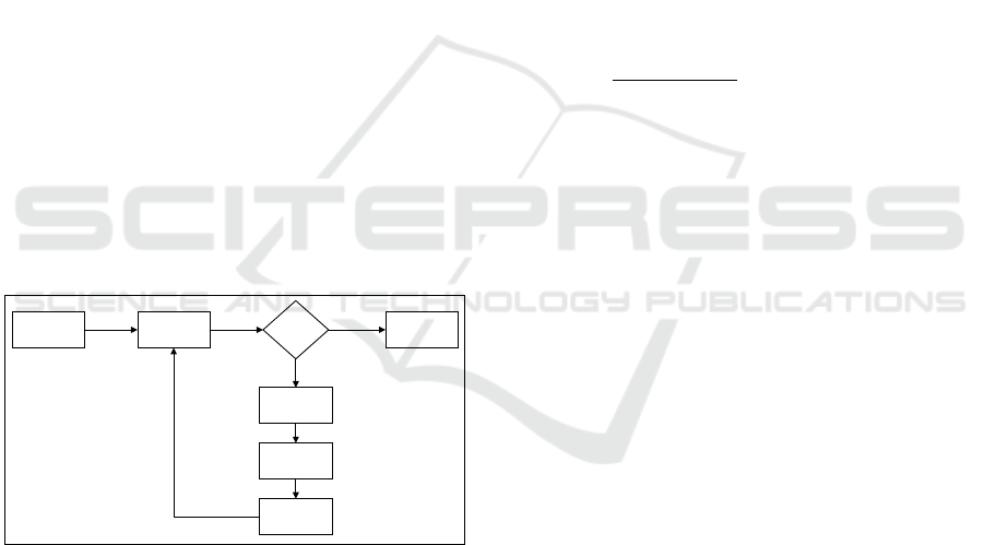
Figure 2: Blockdiagram of the Genetic Algorithm.

4 OPTIMIZATION

Given that the designed controllers are conﬁgured as

Single-Input Single-Output (SISO) systems, tuning

the R parameter in the cost function to adhere to the

speciﬁed passenger comfort criteria is sufﬁcient. This

tuning approach accelerates the optimization process

and reduces computational demands. To ﬁnd the con-

troller parameters, the Genetic Algorithm (GA) opti-

mization method (Mathew, 2012) has been selected.

Its simpliﬁed process is depicted in Figure 2.

The core of the GA starts with the initialization of

a population, which in this paper consisted of 20 in-

dividuals. Each individual, represented as a chromo-

some, encodes a potential solution to the optimization

problem. The diversity within this initial population

is crucial as it affects the ability of the algorithm to ex-

plore different areas of the solution space effectively.

The ﬁtness of each chromosome is assessed based

on its suitability to solve the problem at hand, which,

in this case, was guided by a ﬁtness function deﬁned

as follows:

total

= J

+ J

˙a

+ J

(32)

where J

, J

˙a

, J

and J

are the penalty on lateral ac-

celeration, lateral jerk, lateral deviation, and steering

angle, respectively.

Each term of the ﬁtness function is calculated us-

ing the same equation, which is provided for the lat-

eral acceleration term as an example:

(

t=0

y,max

−|a

if |a

| > a

y,max

0 otherwise

(33)

where W

is a weight derived from Bryson’s rule,

T is the simulation time, and a

y,max

is the maximum

allowed acceleration. The maximum allowed values

have been determined based on the ISO 2631 stan-

dard, the desired tracking accuracy, and the physical

limitations of the steering actuator.

The objective is to minimize oscillations, maxi-

mize the smoothness of the control process, reduce

lateral deviations from the desired path, and control

the peaks in the steering angles. This comprehensive

approach ensures that the optimization enhances com-

fort by smoothing acceleration and jerk and improves

path tracking and steering behavior.

After evaluating the ﬁtness of the population, the

algorithm checks if the stopping condition is met.

This study deﬁned the stopping condition as reaching

a maximum of 60 generations. If the stopping condi-

tion is not met, the algorithm proceeds with the selec-

tion of individuals for the next generation. This selec-

tion is typically based on ﬁtness values, where better-

performing individuals are more likely to be selected,

ensuring that the advantageous traits are carried for-

ward.

The selected individuals then undergo crossover

and mutation processes. Crossover involves combin-

ing pairs of individuals (parents) to produce new in-

dividuals (offspring) by exchanging segments of their

chromosomes, thereby creating diversity while pre-

serving useful genetic information. Mutation intro-

duces random changes to individual chromosomes,

which helps maintain genetic diversity within the

ICINCO 2024 - 21st International Conference on Informatics in Control, Automation and Robotics

population and prevents premature convergence to

suboptimal solutions. Each iteration of this process

determines a new R value based on the current popu-

lation. This value is then used to re-evaluate the ﬁt-

ness function in the next iteration. This iterative pro-

cess continues until the ﬁtness function converges to

an optimal solution, ensuring that the GA effectively

tunes the R parameter to meet the speciﬁed passenger

comfort criteria.

5 SIMULATION ENVIRONMENT

The control algorithms and optimization processes

have been implemented in the Matlab/Simulink en-

vironment. The simulation environment has been cre-

ated in the CarMaker software package. It has been

chosen for its ability to simulate real-world conditions

accurately and its well-deﬁned Matlab interface.

Table 1: Vehicle Parameters.

Parameter Symbol Value Unit

Mass m 1463 [kg]

Inertia I

1600 [kg · m

]

Distance from CoM to

front axle

1.1 [m]

Distance from CoM to

rear axle

1.58 [m]

Front cornering stiffness C

a f

80000 [N/rad]

Rear cornering stiffness C

80000 [N/rad]

For the simulations, the default vehicle model of

CarMaker has been used, whose parameters are listed

in Table 1. The lateral acceleration and path deviation

have been measured using built-in inertial and road

sensors. The jerk was computed by differentiating the

acceleration and applying a low-pass ﬁlter to reduce

noise resulting from numerical differentiation.

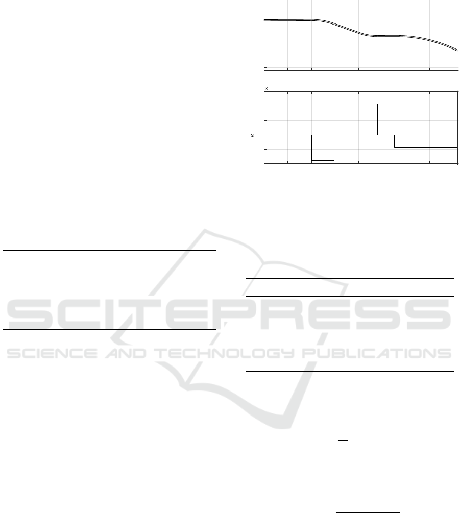
The test case consists of a suburban road section,

which has been designed for a maximum 50 km/h ve-

hicle speed. Figure 3 illustrates the turning radius

and trajectory. According to (Kilinc and Baybura,

2012) and (Jagel

ak et al., 2022), the ideal road radius

ranges between 230 m and 280 m, which corresponds

to a lateral acceleration of 1.47 m/s

. Consequently,

the curvatures of the road correspond to 230 m and

280 m turning radius.

6 RESULTS

Several key metrics have been considered to facili-

tate a comprehensive comparison. Based on (Luciani

et al., 2020) and the ISO 2631 standard, the equivalent

acceleration (a

) and the MSDV value have been se-

lected as metrics of passenger comfort. Based on the

0 100 200 300 400 500 600 700 800 900

-200

-100

Y [m]

0 100 200 300 400 500 600 700 800 900

X [m]

-4

-2

-1

]

-3

Figure 3: Desired path and road curvature.

likely passenger comfort, the equivalent acceleration

has been divided into different categories, shown in

Table 2.

Table 2: Likely reactions to various magnitudes of overall

vibration total values, speciﬁed in ISO 2631-1.

[m/s

] Reaction

≤ 0.315 Not uncomfortable

0.315 ≤ a

≤ 0.63 A little uncomfortable

0.5 ≤ a

≤ 1 Fairly uncomfortable

0.8 ≤ a

≤ 1.6 Uncomfortable

1.25 ≤ a

≤ 2.5 Very uncomfortable

≥ 2 Extremely uncomfortable

To determine the equivalent acceleration, ﬁrst, the

frequency-weighted root mean square (WRMS) ac-

celeration along the main axes is calculated as:

,RMS



(t)dt



(34)

where T

represents the integration time, a

is the

frequency-weighted function, and a

,RMS

is the root

mean square of a

Then, the equivalent acceleration can be calcu-

lated as:

x,W

+ k

y,W

(35)

Here, a

x,W

and a

y,W

are the frequency-weighted

RMS accelerations along the x and y axes, respec-

tively, and k

and k

are weighting factors. Assuming

= k

= 1 and neglecting the longitudinal acceler-

ation (as the longitudinal acceleration has been con-

stant), a

can be calculated as the RMS of a

y,W

over

the entire track.

The second index evaluated is the Motion Sick-

ness Dose Value (MSDV), which describes the proba-

Comparison of Lateral Controllers for Autonomous Vehicles Based on Passenger Comfort Optimization

bility of motion sickness occurrence due to oscillatory

motion. This index is calculated similarly to a

but

uses W

as the frequency-weighted function. Accord-

ing to the ISO 2631 standard, the likelihood of nausea

symptoms is calculated as follows:

MSDV

[%] =

· a

MSDV

× 100 (36)

Furthermore, the performance of the controllers

with respect to reference signal tracking and the con-

trol input has also been evaluated beyond passenger

comfort.

0 20 40 60 80 100 120 140

-2

LQR

0 20 40 60 80 100 120 140

-2

Lateral acceleration [m/s²]

LQ-Servo

0 20 40 60 80 100 120 140

Time [s]

-2

MPC

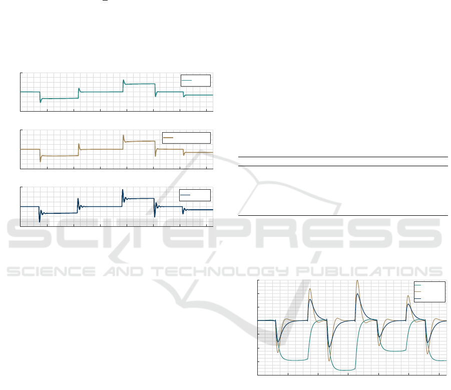
Figure 4: Lateral acceleration of the vehicles at 50 km/h.

As depicted in Figure 4, the observed peaks in ac-

celeration are primarily the result of sudden changes

in cornering. These peaks vary signiﬁcantly among

different controllers. In the case of the LQR, the peaks

are conﬁned within smaller limits due to the nature of

the control strategy. Conversely, the other two con-

trollers show larger acceleration peaks due to their in-

tegrating characteristics.

A more detailed examination of the controller per-

formance metrics is presented in Table 3. The data in-

dicates that all three controllers are in the ’not uncom-

fortable’ category with respect to equivalent accelera-

tion (a

). This observation indicates a relatively uni-

form level of performance among the controllers con-

cerning passenger comfort across the entire track.

In particular, the LQR and LQ-Servo controllers

showed comparable a

values, underscoring a con-

sistent response to dynamic vehicular motions. In

contrast, the Model Predictive Control (MPC) demon-

strated slightly elevated a

values.

Considering the MSDV values, all three con-

trollers achieved approximately 4%, which complies

with the regulations.

Regarding the magnitude of the acceleration

peaks, the maximum values were most signiﬁcant

in the MPC controller, nearly one and ﬁfty percent

greater than those observed with the LQR. This high-

lights the higher responsiveness of the MPC con-

troller, which is caused by the augmentation of the

modiﬁed dynamic bicycle model.

The controllers have also been tested on the same

track at 70 km/h and 100 km/h speeds. The results

of these tests are presented in Table 4. It can be ob-

served that the maximum absolute acceleration and

MSDV values increase signiﬁcantly as the curvature

has been deﬁned for a lower maximum speed. How-

ever, in terms of equivalent acceleration (a

), even at

100 km/h, only the MPC controller falls in the middle

of the ”a little uncomfortable” range, while the other

two controllers are near the bottom of this range, al-

most reaching the ”not uncomfortable” category.

Table 3: Controller performance comparison at 50 km/h.

Metric LQR LQ-Servo MPC

[m/s

] 0.090642 0.096871 0.11723

MSDV

[%] 3.9759 3.9034 4.0441

peak

[m/s

] 1.193 1.42 1.752

Maximal Jerk [m/s

] 6.63 10.77 13.96

Average / maximal Lateral

Deviation [m]

0.0295 / 0.0731 0.0071 / 0.0594 0.007 / 0.0395

Input signal settling time [s] 0.376 0.426 0.837

While peak accelerations were associated with

corresponding increases in jerk magnitudes, higher

jerk does not necessarily equate to poorer passenger

comfort, according to (de Winkel et al., 2023).

20 40 60 80 100 120 140

Time [s]

-0.08

-0.06

-0.04

-0.02

0.02

0.04

0.06

Lateral deviation [m]

LQR

LQ-Servo

MPC

Figure 5: Comparison of the lateral deviations.

As Figure 5 shows, the LQR controller does not

reduce the steady-state error due to its lack of an in-

tegrating component. In contrast, although it shows

larger transient deviations, the LQ-Servo controller

effectively reduces this error to zero. This behav-

ior is attributed to the integrating element within the

LQ-Servo controller, designed to correct long-term

steady-state errors. However, the initial reduction and

subsequent overshoot of integrated errors can lead to

a delayed response from the controller. The MPC per-

forms best in terms of tracking accuracy. Speciﬁcally,

ICINCO 2024 - 21st International Conference on Informatics in Control, Automation and Robotics

it achieves an order of magnitude smaller maximum

lateral deviation over the entire track compared to the

LQR controller.

The MPC is tuned to be the most aggressive,

resulting in the longest control signal settling time

among the controllers.

Table 4: Controller performance comparison at different

speeds.

Metric LQR LQ-Servo MPC

50 km/h

[m/s

] 0.090642 0.096871 0.11723

MSDV

[%] 3.9759 3.9034 4.0441

Max absolute a

[m/s

] 1.2421 1.4737 1.7523

70 km/h

[m/s

] 0.18601 0.18636 0.23495

MSDV

[%] 10.5429 10.6457 10.5926

Max absolute a

[m/s

] 2.3904 2.427 3.0725

100 km/h

[m/s

] 0.35503 0.37098 0.52087

MSDV

[%] 22.9865 23.5348 22.5547

Max absolute a

[m/s

] 3.8248 3.9982 5.6173

7 CONCLUSION

This paper compared three model-based controllers

in terms of lateral acceleration and jerk as indicators

of passenger comfort and reference signal tracking.

These properties were optimized using a genetic algo-

rithm to ensure the controllers met the speciﬁed crite-

ria. All three controllers complied with the standards

described in the relevant regulations.

All three controllers achieved low reference track-

ing errors while meeting passenger comfort require-

ments for the given tracking bicycle model and the

speciﬁed simulation vehicle on the designated track.

Considering overall performance, including equiva-

lent acceleration, MSDV, lateral deviation, jerk, and

input signal settling time, the LQ-Servo controller

proved the most optimal. Although it slightly under-

performed compared to the MPC in reference track-

ing, it demonstrated twice as fast settling times and

20% lower peak accelerations, making it the best

choice in this simulation and model structure. Also,

the a

were lower, especially at higher speeds.

These results suggest that the LQ-Servo controller

could be a promising option for real vehicle tests.

In future work, the integration of machine learning

methods with classical controllers for lateral vehicle

control will be considered. The robustness of these

algorithms against parametric uncertainties, such as

shifts in the center of mass, payload changes, and

tire variations, will be evaluated. Additionally, their

performance in handling lateral disturbances like side

wind gusts will be analyzed, with a focus on both ve-

hicle stability and passenger comfort, including the

potential for motion sickness.

ACKNOWLEDGEMENTS

This work was supported by the European Union

within the framework of the National Laboratory for

Autonomous Systems (RRF-2.3.1-21-2022-00002).

REFERENCES

AbdElmoniem, A., Osama, A., Abdelaziz, M., and

Maged, S. A. (2020). A path-tracking algo-

rithm using predictive stanley lateral controller. In-

ternational Journal of Advanced Robotic Systems,

17(6):1729881420974852.

Athans, M. and Falb, P. L. (2013). Optimal control: an in-

troduction to the theory and its applications. Courier

Corporation.

Cascetta, E., Carteni, A., and Di Francesco, L. (2022). Do

autonomous vehicles drive like humans? a turing ap-

proach and an application to sae automation level 2

cars. Transportation research part C: emerging tech-

nologies, 134:103499.

de Winkel, K. N., Irmak, T., Happee, R., and Shyrokau, B.

(2023). Standards for passenger comfort in automated

vehicles: Acceleration and jerk. Applied Ergonomics,

106:103881.

asp

ar, P., Szab

o, Z., Bokor, J., and N

emeth, B. (2016).

Robust control design for active driver assistance sys-

tems. Springer, Book, 10:978–3.

Jagel

ak, J., Gnap, J., Kuba, O., Frnda, J., and Kostrzewski,

M. (2022). Determination of turning radius and lateral

acceleration of vehicle by gnss/ins sensor. Sensors,

22(6):2298.

Kilinc, A. S. and Baybura, T. (2012). Determination of min-

imum horizontal curve radius used in the design of

transportation structures, depending on the limit value

of comfort criterion lateral jerk. TS06G-Engineering

Surveying, Machine Control and Guidance.

Li, D., Zhao, D., Zhang, Q., and Chen, Y. (2019). Re-

inforcement learning and deep learning based lat-

eral control for autonomous driving [application

notes]. IEEE Computational Intelligence Magazine,

14(2):83–98.

Luciani, S., Bonﬁtto, A., Amati, N., and Tonoli, A. (2020).

Model predictive control for comfort optimization in

assisted and driverless vehicles. Advances in Mechan-

ical Engineering, 12(11):1687814020974532.

Mashadi, B., Mahmoudi-Kaleybar, M., Ahmadizadeh,

P., and Oveisi, A. (2014). A path-following

driver/vehicle model with optimized lateral dynamic

controller. Latin American journal of solids and struc-

tures, 11:613–630.

Mathew, T. V. (2012). Genetic algorithm. Report submitted

at IIT Bombay, 53.

Menhour, L., Lechner, D., and Charara, A. (2012). De-

sign and experimental validation of linear and nonlin-

ear vehicle steering control strategies. Vehicle system

dynamics, 50(6):903–938.

Comparison of Lateral Controllers for Autonomous Vehicles Based on Passenger Comfort Optimization

Mesghali, K. (2021). Control tuning of autonomous

vehicles considering performance-comfort trade-offs.

Master’s thesis, School of Industrial and Information

Engineering.

Moreno-Gonzalez, M., Artu

nedo, A., Villagra, J., Join, C.,

and Fliess, M. (2022). Speed-adaptive model-free lat-

eral control for automated cars. IFAC-PapersOnLine,

55(34):84–89.

emeth, B. and G

asp

ar, P. (2011). Road inclinations in the

design of LPV-based adaptive cruise control∗. IFAC

Proceedings Volumes, 44(1):2202–2207.

Poussot-Vassal, C., Sename, O., Dugard, L., and Savaresi,

S. (2011). Vehicle dynamic stability improvements

through gain-scheduled steering and braking control.

Vehicle System Dynamics, 49(10):1597–1621.

Rajamani, R. (2011). Vehicle dynamics and control.

Springer Science & Business Media.

Samuel, M., Hussein, M., and Mohamad, M. B. (2016). A

review of some pure-pursuit based path tracking tech-

niques for control of autonomous vehicle. Interna-

tional Journal of Computer Applications, 135(1):35–

38.

Sever, M., Zengin, N., Kirli, A., and Arslan, M. S. (2021).

Carsickness-based design and development of a con-

troller for autonomous vehicles to improve the com-

fort of occupants. Proceedings of the Institution of

Mechanical Engineers, Part D: Journal of Automobile

Engineering, 235(1):162–176.

Tagne, G., Talj, R., and Charara, A. (2015). Design

and comparison of robust nonlinear controllers for

the lateral dynamics of intelligent vehicles. IEEE

Transactions on Intelligent Transportation Systems,

17(3):796–809.

oth, R. (2010). Modeling and identiﬁcation of linear

parameter-varying systems, volume 403. Springer.

Wang, L. (2009). Model predictive control system de-

sign and implementation using MATLAB, volume 3.

Springer.

Zhang, Y., Sun, P., Yin, Y., Lin, L., and Wang, X. (2018).

Human-like autonomous vehicle speed control by

deep reinforcement learning with double q-learning.

In 2018 IEEE intelligent vehicles symposium (IV),

pages 1251–1256. IEEE.

Zhu, M., Wang, X., and Wang, Y. (2018). Human-

like autonomous car-following model with deep rein-

forcement learning. Transportation research part C:

emerging technologies, 97:348–368.

Zin, A., Sename, O., Gaspar, P., Dugard, L., and Bokor,

J. (2008). Robust LPV-H ∞ control for active sus-

pensions with performance adaptation in view of

global chassis control. Vehicle System Dynamics,

46(10):889–912.

ICINCO 2024 - 21st International Conference on Informatics in Control, Automation and Robotics