Triplet Neural Networks for the Visual Localization of Mobile Robots
Marcos Alfaro
1 a
, Juan Jos
´
e Cabrera
1 b
, Luis Miguel Jim
´
enez
1 c
,
´
Oscar Reinoso
1,2 d
and Luis Pay
´
a
1 e
1
Engineering Research Institute of Elche (I3E), Miguel Hernandez University, Elche, Spain
2
ValgrAI: Valencian Graduate School and Research Network of Artificial Intelligence, Valencia, Spain
Keywords:
Robot Localization, Panoramic Images, Convolutional Neural Network, Triplet Loss.
Abstract:
Triplet networks are composed of three identical convolutional neural networks that function in parallel and
share their weights. These architectures receive three inputs simultaneously and provide three different out-
puts, and have demonstrated to have a great potential to tackle visual localization. Therefore, this paper
presents an exhaustive study of the main factors that influence the training of a triplet network, which are the
choice of the triplet loss function, the selection of samples to include in the training triplets and the batch size.
To do that, we have adapted and retrained a network with omnidirectional images, which have been captured
in an indoor environment with a catadioptric camera and have been converted into a panoramic format. The
experiments conducted demonstrate that triplet networks improve substantially the performance in the visual
localization task. However, the right choice of the studied factors is of great importance to fully exploit the
potential of such architectures.
1 INTRODUCTION
Vision systems are a very suitable option to tackle
mobile robot localization. This type of sensors is able
to capture rich information from the scene, such as
colors, textures and shapes. Inside this group, om-
nidirectional cameras stand out (Flores et al., 2024).
Since they have a wide field of view and they capture
the same information independently of the robot ori-
entation, a complete map of the environment can be
built with a fairly small number of images.
To build a map of the environment, which can be
used by the robot to estimate its position, visual in-
formation must be processed and compressed. Global
description consists in obtaining a unique descriptor
per image that contains the essential information of
the image (Cebollada et al., 2019). Nowadays, these
descriptors are mostly obtained with CNNs.
Convolutional Neural Networks (CNNs) are com-
posed of layers that apply the convolution operation to
the input image, being able to extract features with a
a
https://orcid.org/0009-0008-8213-557X
b
https://orcid.org/0000-0002-7141-7802
c
https://orcid.org/0000-0003-3385-5622
d
https://orcid.org/0000-0002-1065-8944
e
https://orcid.org/0000-0002-3045-4316
high level of abstraction (Benyahia et al., 2022). This
ability makes them especially useful to obtain robust
image descriptors and subsequently to build a map of
the environment.
Frequently, CNNs are trained with more complex
architectures, composed of several branches that work
in parallel. That is the case of siamese and triplet net-
works, which contain two and three identical CNNs,
respectively. These architectures are able to learn
similarities and differences amongst the input data.
Triplet networks are trained with combinations of
three images, called anchor (I
a
), positive (I
+
) and
negative (I
−
). When it comes to visual localization,
triplet samples must be chosen in such a way that the
anchor and the positive images must be captured from
a similar position of the target environment, whereas
the negative image must be captured from a different
position (see Figure 1).
With the aim of maximizing their performance,
several factors must be considered regarding the train-
ing process. One is the choice of the triplet loss func-
tion, which can be defined as a mathematical func-
tion that receives the output of each network and cal-
culates the error committed by the model (Hermans
et al., 2017). Depending on this error, the optimizer
algorithm will update the weights of the network to a
greater or lesser degree.
Alfaro, M., Cabrera, J., Jiménez, L., Reinoso, Ó. and Payá, L.
Triplet Neural Networks for the Visual Localization of Mobile Robots.
DOI: 10.5220/0012927400003822
Paper published under CC license (CC BY-NC-ND 4.0)
In Proceedings of the 21st International Conference on Informatics in Control, Automation and Robotics (ICINCO 2024) - Volume 2, pages 125-132
ISBN: 978-989-758-717-7; ISSN: 2184-2809
Proceedings Copyright © 2024 by SCITEPRESS – Science and Technology Publications, Lda.
125

Figure 1: Complete training process of a triplet network. I
a
, I
+
and I
−
are the anchor, positive and negative images, whereas
⃗
d
a
,
⃗
d
+
and
⃗
d
−
are their respective descriptors.
Regarding the selection of the triplet samples, it is
not an intuitive task in a global localization approach.
Although some environments can be discretized into
a finite number of classes (for example, indoor envi-
ronments are usually divided into rooms), another cri-
terion must be followed if a fine-grained estimation of
the robot pose is required.
To speed up the training process, images are
loaded into the network as small packages called
batches. From every batch, the loss function calcu-
lates the error committed for each triplet sample and
returns a unique error, that can be either the average
value, the maximum or a more complex function.
In this paper we address robot localization with a
CNN, which is adapted and trained by employing a
triplet architecture. The network is trained with om-
nidirectional images that have been previously con-
verted into a panoramic format. Furthermore, we
present an exhaustive evaluation of the most impor-
tant factors that influence the training of a CNN while
employing a triplet architecture, that is, the triplet loss
function, the batch size and the choice of the triplet
samples for the network training. All of these factors
are analyzed to optimize the learning process of the
CNN in the visual localization task.
This manuscript is structured as follows. Section 2
reviews the state of the art of visual localization with
CNNs. The proposed architecture is detailed in Sec-
tion 3, whereas the localization approach is described
in Section 4. Section 5 collects the experiments con-
ducted in this work and the results obtained for each
of them. These results are compared to other ap-
proaches in Section 6. Finally, in Section 7 we discuss
the results obtained and future works are proposed.
2 PREVIOUS WORK
This section outlines the state of the art of visual lo-
calization with CNNs. Section 2.1 describes the ap-
proaches that addressed this problem with architec-
tures composed of a unique network, whereas Section
2.2 analyzes the works that employed triplet architec-
tures.
2.1 Localization with CNNs
In recent years, CNNs have become a common choice
to tackle visual localization. In this scope, these
networks are typically employed to obtain global-
appearance descriptors from an image (Arroyo et al.,
2016). Besides, they can also be used to estimate di-
rectly the coordinates where an image has been cap-
tured, by employing regression layers (Foroughi et al.,
2021).
Some works have sought to exploit the advantages
of omnidirectional vision with CNNs. In this sense,
(Rostkowska and Skrzypczy
´
nski, 2023) tackle indoor
localization with a global-appearance approach.
2.2 Localization with Triplet Networks
Due to the success of CNNs, several approaches have
explored the use of more complex architectures dur-
ing the training of a CNN, that is, siamese networks
(Cabrera et al., 2024) and triplet networks (Brosh
et al., 2019). Triplet architectures contain three iden-
tical networks that work in parallel, and it has been
proved that they have a great potential to address this
task and can outperform simple CNNs or siamese ar-
chitectures (Olid et al., 2018).
With the rise of triplet networks, some authors
have focused on the design of triplet loss functions,
which have been evaluated in different tasks such as
people reidentification (Hermans et al., 2017) or place
recognition with lidar (Uy and Lee, 2018).
All in all, since triplet architectures have demon-
strated to have a great potential to tackle visual local-
ization, an evaluation of the main factors that influ-
ence the training process of the CNN is necessary.
ICINCO 2024 - 21st International Conference on Informatics in Control, Automation and Robotics
126

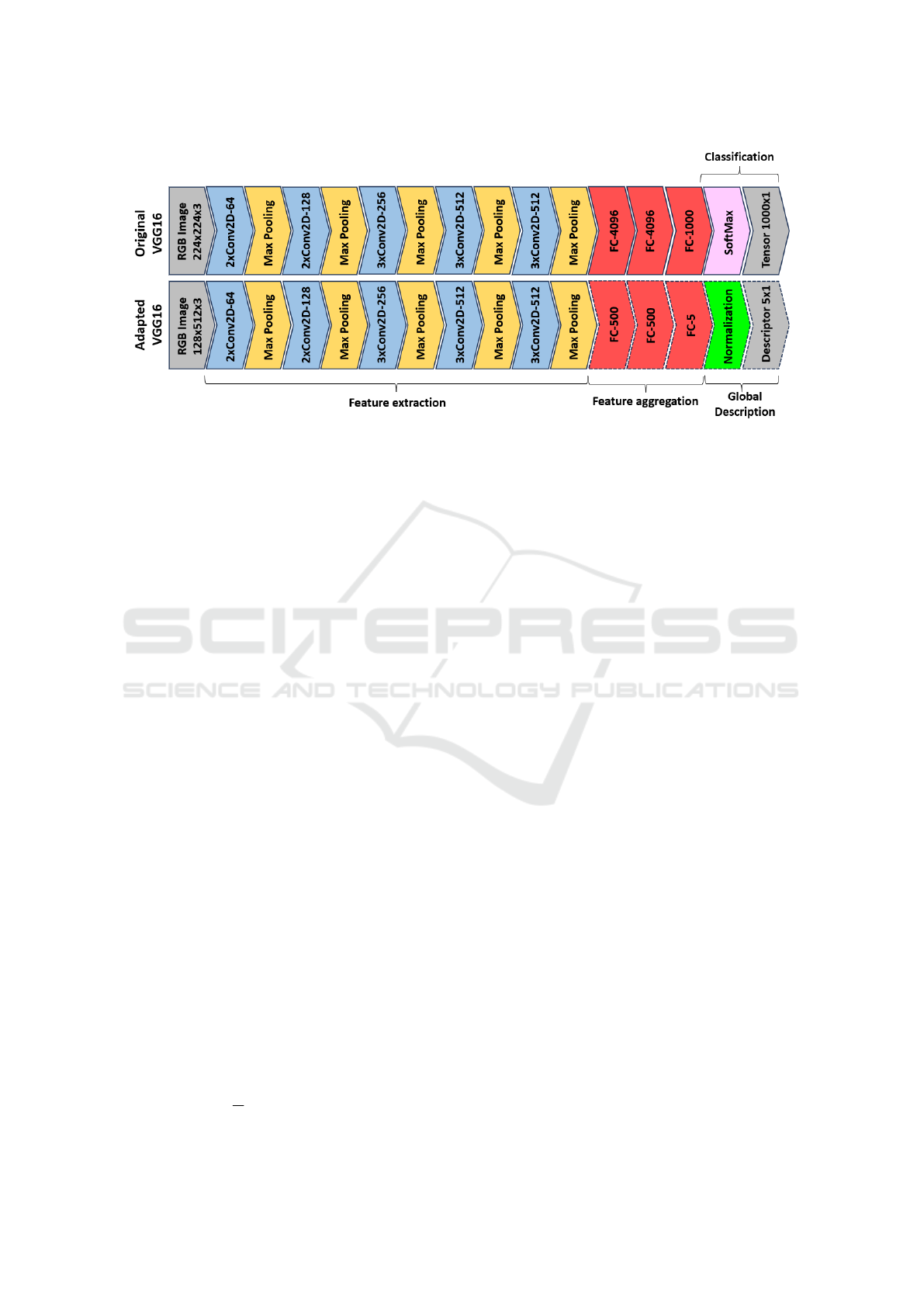
Figure 2: Architecture of the VGG16 network: original (above) and our adaptation (below). To simplify the diagrams, ReLU
layers have not been included.
3 TRIPLET NETWORK
3.1 Proposed Architecture
In this work, a CNN is adapted and trained by em-
ploying a triplet architecture. The literature reviewed
in Section 2 proves that these networks are especially
suitable to tackle visual localization.
The network model that we have employed is
VGG16 (Simonyan and Zisserman, 2014), since it has
demonstrated to have a great potential in a similar
task (Cabrera et al., 2024). This architecture has been
adapted as shown in Figure 2. The convolutional lay-
ers have been left intact, whereas the fully connected
layers have been modified so as to adapt the network
to the size of the input image and to obtain a global
descriptor with size 5x1.
To leverage the ability of the VGG16 architecture
to extract features from the input images, the transfer
learning technique has been employed in the convolu-
tional layers, whereas the fully connected layers have
been trained from scratch.
3.2 Triplet Loss Functions
In this work, a comparative evaluation of different
triplet losses is conducted in Experiment 1, which are
presented below. Table 1 includes the definitions of
all the terms employed to formulate the loss functions.
• Triplet Margin Loss (TL): it is the most
renowned triplet loss. It returns the average error
of all the batch combinations:
L =
1
N
N
∑
i=1
[D
i
a,p
− D
i
a,n
+ m]
+
• Lazy Triplet Loss (LT): similar to the Triplet
Margin Loss, but it returns the maximum error of
the entire batch instead of the average:
L =
h
max

⃗
D
a,p
−
⃗
D
a,n
+ m
i
+
• Circle Loss (CL): introduced in (Sun et al.,
2020), it includes two parameters that must be ad-
justed (γ and m). Instead of Euclidean distance, it
makes use of the cosine similarity metric:
L = ln 1 +
N
∑
j=1
e
γ α
j
n
s
j
n
+
N
∑
i=1
e
−γ α
i
p
s
i
p
!
where:
α
i
p
=

O
p
− s
i
p

+
;α
j
n
=

s
j
n
− O
n

+
O
p
= 1 − m; O
n
= m
• Angular Loss (AL): proposed by (Wang et al.,
2017), it seeks to minimize the angle formed by
the anchor and the negative descriptors and the
angle formed by the positive and the negative de-
scriptors:
L = ln 1 +
N
∑
i=1
e
f
i
a,p,n
!
where:
f
i
a,p,n
= 4tan
2
α

x
i
a
+ x
i
p

T
x
i
n
− 2

1 + tan
2
α

x
i
T
a
x
i
p
Triplet Neural Networks for the Visual Localization of Mobile Robots
127

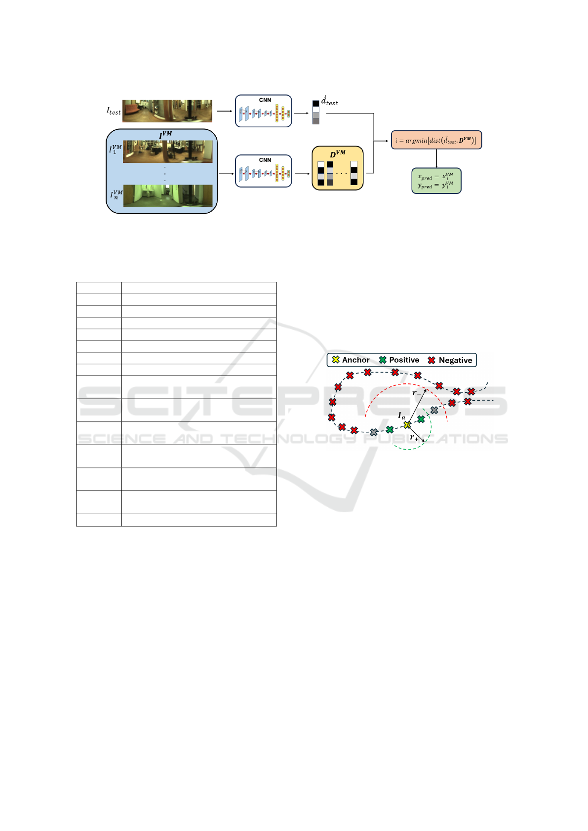
Figure 3: Test process, where each image descriptor
⃗
d
test
is compared with the descriptors of all the images of the visual
model D
V M
=
h
⃗
d
V M
1
,
⃗
d
V M
2
,...,
⃗
d
V M
n
i
. The nearest neighbour will indicate the estimated robot coordinates (x
pred
,y
pred
).
Table 1: Symbology employed in the definition of the triplet
loss functions.
Symbol Description
L Loss error
N Batch size
[...]
+
ReLU function
m Margin
γ Scale factor
α Angular margin
a, p, n Anchor, positive and negative inputs
D
i
a,p
Euclidean distance between the
descriptors a and p of the i-th triplet
D
i
a,n
Euclidean distance between the
descriptors a and n of the i-th triplet
⃗
D
a,p
Euclidean distances between
each a-p pair from a batch
⃗
D
a,n
Euclidean distances between
each a-n pair from a batch
s
i
p
Cosine similarity between the
descriptors a and p of the i-th triplet
s
j
n
Cosine similarity between the
descriptors a and n of the j-th triplet
x
i
a
,x
i
p
,x
i
n
descriptors a, p, n of the i-th triplet
4 VISUAL LOCALIZATION
In order to address the localization problem, we have
used omnidirectional images captured with a cata-
dioptric vision system, which is mounted on a mo-
bile robot. Next, the images have been converted
into a panoramic format with a size of 128x512 pixels
(RGB). Afterwards, the initial set of images has been
split into training, validation and test sets.
Concerning the training process, a triplet archi-
tecture is used. The coordinates where each image
has been captured are available, which enables us to
train the CNN in a supervised fashion. The network
receives combinations of three images (I
a
,I
p
,I
n
) and
outputs three different descriptors (
⃗
d
a
,
⃗
d
p
,
⃗
d
n
). These
combinations are chosen randomly, in such a way that
the anchor and the positive images must have been
captured within a threshold distance called r
+
, and the
distance between the anchor and the negative images
must be bigger than a threshold called r
−
(see Figure
4). In Experiment 2, the influence of these thresholds
on the network performance is studied.
Figure 4: Explanation of the method to select a training
sample with a triplet architecture.
To validate and test the trained model (see Figure
3), each test image I
test
is embedded into a descrip-
tor
⃗
d
test
. Subsequently, this descriptor is compared
with all the image descriptors of the visual model
D
V M
=
h
⃗
d
V M
1
,
⃗
d
V M
2
,...,
⃗
d
V M
n
i
, composed of the im-
ages of the training set.
To compare the descriptors, the metrics that have
been employed are the Euclidean distance, if the net-
work has been trained with the Triplet Margin Loss or
the Lazy Triplet Loss, or the cosine similarity, if the
network has been trained with the Circle Loss or the
Angular Loss.
The capture point of the image whose descriptor
has the minimum Euclidean distance or the maximum
cosine similarity with the test image will be used as
the predicted position of the robot (x
pred
,y
pred
). In
other words, the nearest neighbour will be the estima-
tion of the coordinates where the test image has been
captured.
ICINCO 2024 - 21st International Conference on Informatics in Control, Automation and Robotics
128

5 EXPERIMENTS
This section presents the experiments conducted in
this work. Experiment 1 consists in a comparative
evaluation of several triplet loss functions. Experi-
ment 2 focuses on the optimization of the threshold
values r
+
and r
−
employed for the selection of the
triplet samples. Finally, Experiment 3 analyzes the in-
fluence of the batch size on the network performance
and the computing time.
5.1 Dataset
To address this work, images from COLD-
Freiburg database have been employed (Prono-
bis and Caputo, 2009), which are available from
https://www.cas.kth.se/COLD/. This dataset contains
omnidirectional images that have been captured with
a catadioptric camera mounted on a mobile robot.
The robot follows a path inside a building, going
through different rooms: office rooms, a kitchen, a
toilet or a corridor, among others. Moreover, the
images have been captured under three different
lighting conditions: cloudy, night and sunny.
All of this makes this dataset a perfect option to
validate our method. Figures 5 and 6 show exam-
ples of an omnidirectional image from the COLD-
Freiburg dataset and the same image converted into
a panoramic format, respectively.
Figure 5: Original omnidirectional image from the COLD-
Freiburg dataset. Size = 480×640x3 RGB.
Figure 6: Image converted into a panoramic format. Size =
128×512x3 RGB.
Table 2 shows the sequences that have been used
to conduct the experiments. Only images captured
under cloudy conditions have been employed during
the training and the validation of the network. Be-
sides, the sequence employed in the network training
has been sampled, in such a way that the 20% of the
images are used in training, another 20% are used for
validation and the rest is discarded. Meanwhile, the
networks have been tested under every lighting con-
dition: cloudy, night and sunny.
Table 2: Size and lighting conditions of the training, vali-
dation and test sets. (S) means that the sequence has been
sampled and (C) means that the sequence is complete.
Image set Sequence Images
Training / Visual Model seq2 cloudy3 (S) 588
Validation seq2 cloudy3 (S) 586
Test 1 seq2 cloudy2 (C) 2595
Test 2 seq2 night2 (C) 2707
Test 3 seq2 sunny2 (C) 2114
5.2 Experiment 1: Evaluation of the
Triplet Loss Function
In this experiment, a comparative evaluation amongst
different triplet loss functions, which are defined in
Section 3.2, has been performed. To do so, a network
has been trained with each loss. In every experiment,
the training consists of 10 epochs, with an epoch
length of 25000 triplet samples, and the optimizer al-
gorithm that has been employed is the Stochastic Gra-
dient Descent (SGD).
Table 3 shows the geometric error committed in
the localization process. This error has been measured
as the distance between the coordinates of the test im-
age (x
test
,y
test
), i.e., the ground truth, and the coor-
dinates of the retrieved image (x
pred
,y
pred
) obtained
after the visual localization process (Fig. 3). Since
the robot followed different paths when capturing the
training and the test sequences, the error cannot be
zero. Table 4 shows the minimum error that can be
reached under each lighting condition. Besides, Fig-
ure 7 shows the Recall@K obtained with each triplet
loss function.
Table 3: Geometric error committed with each loss function
in Experiment 1.
Experiment 1 Geometric Error (m)
Loss Function Cloudy Night Sunny Average
TL (m=1) 0.303 0.324 0.633 0.420
LT (m=1.25) 0.266 0.286 0.766 0.439
CL (γ=1, m=1) 0.428 0.547 1.219 0.731
AL (α=30º) 0.338 0.413 0.734 0.495
Table 4: Minimum reachable error under each lighting con-
dition considering the distribution of the test and training
images on the floor plane.
Cloudy Night Sunny Average
Min. Error (m) 0.127 0.126 0.119 0.124
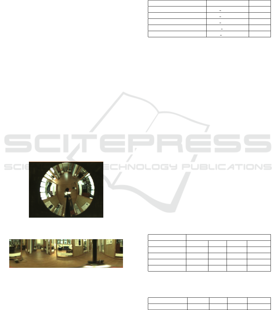
Table 3 and Figure 7 reveal that the best over-
all performance was obtained with the Triplet Mar-
gin Loss (m = 1), followed by the Lazy Triplet Loss
Triplet Neural Networks for the Visual Localization of Mobile Robots
129

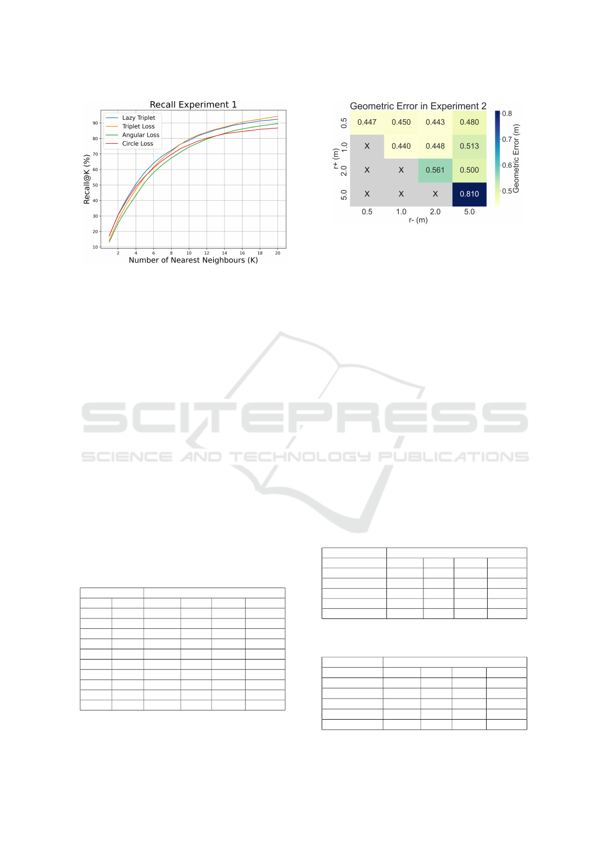
Figure 7: Recall@K obtained with each loss function in
Experiment 1.
(m = 1.25). Despite the fact that the errors are rel-
atively small, considering the size of the building, it
can be noticed that the error committed under sunny
conditions is larger comparing to cloudy and night.
This happens because only cloudy images were used
during the training process. Since sunny is the most
differing condition, the trained network may have ex-
perienced some overfitting to the training condition.
5.3 Experiment 2: Evaluation of the
Triplet Sample Selection
Next, we have analyzed the way we select the triplet
samples that are used during the network training. We
have modified the thresholds r
+
and r
−
, defined in
Section 4 (see Figure 4). The loss function that has
been used is Triplet Margin Loss (m = 1). Table 5
shows the geometric error committed with every com-
bination of threshold values. Meanwhile, Figure 8
shows the heatmap with the average error obtained in
each case.
Table 5: Geometric error committed with each threshold
values in Experiment 2.
Experiment 2 Geometric Error (m)
r
+
(m) r
−
(m) Cloudy Night Sunny Average
0.5 0.5 0.332 0.322 0.687 0.447
0.5 1 0.306 0.335 0.710 0.450
0.5 2 0.306 0.317 0.705 0.443
0.5 5 0.431 0.377 0.632 0.480
1 1 0.358 0.345 0.618 0.440
1 2 0.318 0.351 0.676 0.448
1 5 0.378 0.371 0.790 0.513
2 2 0.383 0.385 0.916 0.561
2 5 0.365 0.372 0.763 0.500
5 5 0.600 0.564 1.265 0.810
Table 5 and Figure 8 reveal that higher values of
r
+
and r
−
have led to a worst performance. This can
Figure 8: Heatmap with the average geometric error com-
mitted with each threshold values in Experiment 2.
be explained as higher threshold values correspond to
less restrictive examples. However, the difference in
the performance amongst the experiments when em-
ploying low threshold values (r
+
<= 1m, r
−
<=
2m) is not noticeable. That means that the variabil-
ity produced by other features of the training process
is higher than the influence of the studied parameters.
5.4 Experiment 3: Study of the Batch
Size
Finally, we have evaluated the influence of the batch
size (N) on the network training. To do that, we have
trained the VGG16 model with different batch sizes.
Tables 6 and 7 include the geometric error com-
mitted for each batch size with the Triplet Margin
Loss and the Lazy Triplet Loss, respectively. Mean-
while, Figure 9 compares the localization error and
the training time required versus the batch size. All
experiments have been carried out on a NVIDIA
GeForce RTX 3090 GPU with 24 GB.
Table 6: Geometric error committed for each batch size
with the Triplet Margin Loss in Experiment 3.
Experiment 3 Geometric Error (m)
Triplet Margin Cloudy Night Sunny Average
N = 1 0.321 0.328 0.602 0.417
N = 2 0.324 0.316 0.562 0.401
N = 4 0.301 0.324 0.529 0.385
N = 8 0.301 0.320 0.555 0.392
N = 16 0.303 0.324 0.633 0.420
Table 7: Geometric error committed for each batch size
with the Lazy Triplet Loss in Experiment 3.
Experiment 3 Geometric Error (m)
Lazy Triplet Cloudy Night Sunny Average
N = 1 0.395 0.356 0.772 0.508
N = 2 0.327 0.379 0.766 0.491
N = 4 0.312 0.335 0.714 0.454
N = 8 0.300 0.337 0.774 0.470
N = 16 0.266 0.286 0.766 0.439
ICINCO 2024 - 21st International Conference on Informatics in Control, Automation and Robotics
130

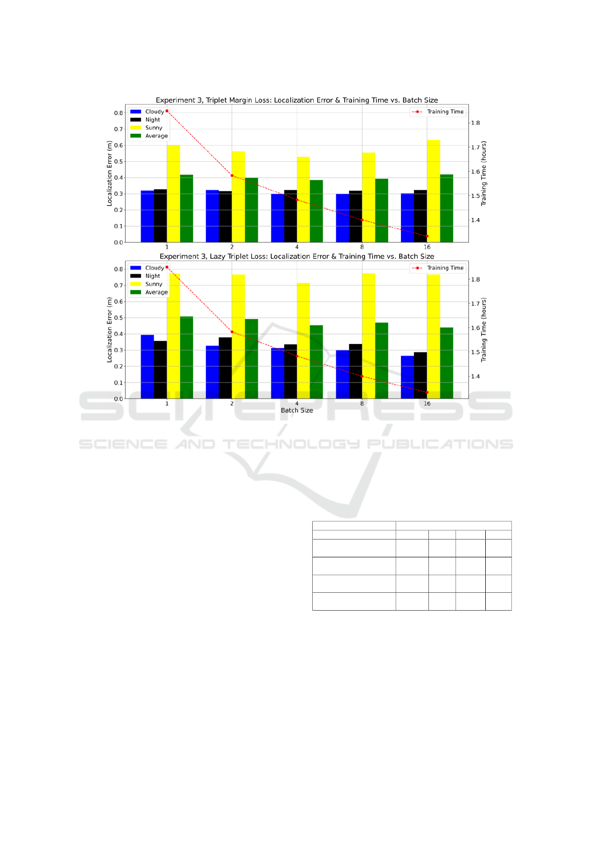
Figure 9: Comparison between the localization error and the training time versus the batch size in Experiment 3, with the
Triplet Margin Loss (above) and the Lazy Triplet Loss (below).
From the results in Experiment 3, it can be ob-
served that the minimum error was obtained with a
batch size N = 4. As expected, the training time
required decreases when the batch size is increased.
It can also be noticed that the Triplet Margin Loss
outperformed the Lazy Triplet Loss with every batch
size.
6 COMPARISON WITH OTHER
WORKS
To evaluate the quality of the proposed method, we
have compared the results obtained with other ap-
proaches that addressed the localization problem with
the COLD database. These works employed global-
appearance descriptors, obtained with analytical tech-
niques (Cebollada et al., 2022) or with CNNs such as
AlexNet (Cabrera et al., 2022). All of these meth-
ods employed only cloudy images to build the visual
model and tested their methods under three different
lighting conditions. They performed a hierarchical lo-
calization, an approach that has demonstrated to be
more accurate. However, it is out of the scope of this
work. Table 8 shows the geometric error obtained by
all the approaches for each lighting condition.
Table 8: Geometric error committed by each approach in
the localization task.
Comparison Geometric Error (m)
Method Cloudy Night Sunny Avg.
Gist
(Cebollada et al., 2022)
0.052 1.065 0.884 0.667
HOG
(Cebollada et al., 2022)
0.163 0.451 0.820 0.478
AlexNet
(Cabrera et al., 2022)
0.293 0.288 0.690 0.424
Triplet VGG16
(ours)
0.301 0.324 0.529 0.385
Under cloudy conditions, some methods em-
ployed a much denser visual model, so the error that
they obtained is lower than the minimum error that
could be reached with our approach (please refer to
Table 4). However, our method obtained a similar
error to the methods that employed the same visual
model (AlexNet). Under sunny conditions, which are
the conditions that most differ from the lighting con-
ditions employed to train the network, our method
Triplet Neural Networks for the Visual Localization of Mobile Robots
131

clearly outperformed the rest of techniques. That
leads to the conclusion that our network was little
affected by overfitting. If all lighting conditions are
taken into account, our method had the best overall
performance.
All in all, although the methods are not directly
comparable, the results demonstrate that employing a
triplet architecture during the training of a CNN im-
proves its performance in the localization task.
7 CONCLUSIONS
Throughout this work, we propose a framework to
perform visual localization with a triplet architecture
and we analyze the main factors that influence the
training process, which are the choice of the triplet
loss function, the triplet sample selection criteria and
the batch size. The experiments reveal that, despite
the fact that triplet architectures have demonstrated
to improve substantially the performance of the net-
work, the right selection of the studied parameters is
a key factor to fully exploit their potential.
In future works, this study could be extended to
outdoor environments, which are much more unstruc-
tured and challenging. Furthermore, we will explore
the use of quadruplet architectures to tackle visual lo-
calization, which are composed of four branches of
CNNs and are able to learn similarities and differ-
ences amongst four images. Finally, we will address
the visual compass problem in order to fully locate
the robot in the floor plane.
ACKNOWLEDGEMENTS
This work is part of the project TED2021-130901B-
I00 funded by MCIN/AEI/10.13039/501100011033
and by the European Union “NextGenera-
tionEU”/PRTR. The work is also part of the
project PROMETEO/2021/075 funded by Generalitat
Valenciana.
REFERENCES
Arroyo, R., Alcantarilla, P. F., Bergasa, L. M., and Romera,
E. (2016). Fusion and binarization of cnn features
for robust topological localization across seasons. In
2016 IEEE/RSJ International Conference on Intelli-
gent Robots and Systems (IROS), pages 4656–4663.
Benyahia, S., Meftah, B., and L
´
ezoray, O. (2022). Multi-
features extraction based on deep learning for skin le-
sion classification. Tissue and Cell, 74:101701.
Brosh, E., Friedmann, M., Kadar, I., Yitzhak Lavy, L., Levi,
E. . . ., and Darrell, T. (2019). Accurate visual local-
ization for automotive applications. In Proceedings
of the IEEE/CVF Conference on Computer Vision and
Pattern Recognition (CVPR) Workshops.
Cabrera, J. J., Cebollada, S., Flores, M., Reinoso,
´
O., and
Pay
´
a, L. (2022). Training, optimization and validation
of a cnn for room retrieval and description of omnidi-
rectional images. SN Computer Science, 3(4):271.
Cabrera, J. J., Rom
´
an, V., Gil, A., Reinoso, O., and Pay
´
a, L.
(2024). An experimental evaluation of siamese neu-
ral networks for robot localization using omnidirec-
tional imaging in indoor environments. Artificial In-
telligence Review, 57(8):198.
Cebollada, S., Pay
´
a, L., Jiang, X., and Reinoso, O. (2022).
Development and use of a convolutional neural net-
work for hierarchical appearance-based localization.
Artificial Intelligence Review, 55(4):2847–2874.
Cebollada, S., Pay
´
a, L., Mayol, W., and Reinoso, O. (2019).
Evaluation of clustering methods in compression of
topological models and visual place recognition us-
ing global appearance descriptors. Applied Sciences,
9(3):377.
Flores, M., Valiente, D., Peidr
´
o, A., Reinoso, O., and Pay
´
a,
L. (2024). Generating a full spherical view by mod-
eling the relation between two fisheye images. The
Visual Computer, pages 1–26.
Foroughi, F., Chen, Z., and Wang, J. (2021). A cnn-based
system for mobile robot navigation in indoor envi-
ronments via visual localization with a small dataset.
World Electric Vehicle Journal, 12(3).
Hermans, A., Beyer, L., and Leibe, B. (2017). In defense
of the triplet loss for person re-identification. arXiv
preprint arXiv:1703.07737.
Olid, D., F
´
acil, J. M., and Civera, J. (2018). Single-
view place recognition under seasonal changes. arXiv
preprint arXiv:1808.06516.
Pronobis, A. and Caputo, B. (2009). Cold: The cosy
localization database. The International Journal of
Robotics Research, 28(5):588–594.
Rostkowska, M. and Skrzypczy
´
nski, P. (2023). Optimizing
appearance-based localization with catadioptric cam-
eras: Small-footprint models for real-time inference
on edge devices. Sensors, 23(14):6485.
Simonyan, K. and Zisserman, A. (2014). Very deep con-
volutional networks for large-scale image recognition.
arXiv preprint arXiv:1409.1556.
Sun, Y., Cheng, C., Zhang, Y., Zhang, C., Zheng, L., Wang,
Z., and Wei, Y. (2020). Circle loss: A unified perspec-
tive of pair similarity optimization. In Proceedings
of the IEEE/CVF conference on computer vision and
pattern recognition, pages 6398–6407.
Uy, M. A. and Lee, G. H. (2018). Pointnetvlad: Deep point
cloud based retrieval for large-scale place recognition.
In Proceedings of the IEEE Conference on Computer
Vision and Pattern Recognition (CVPR).
Wang, J., Zhou, F., Wen, S., Liu, X., and Lin, Y. (2017).
Deep metric learning with angular loss. In Proceed-
ings of the IEEE international conference on com-
puter vision, pages 2593–2601.
ICINCO 2024 - 21st International Conference on Informatics in Control, Automation and Robotics
132