Image Discrimination and Parameter Analysis Based on

Convolutional Neural Networks (CNN)

Jiahan Hu

College of Transportation Engineering, Tongji University, Shanghai, China

Keywords: Deep Learning, Image Classification, Parameter Selection.

Abstract: In the realm of deep learning, various fields benefit from its wide-ranging applications. Image classification

stands out as a classic task in computer vision, demanding meticulous selection of model parameters. The

objective of this study is to investigate how model structure, regularization techniques, and optimizers

influence model performance and identify the optimal configuration from available options. The research

compares the accuracy fluctuations of two model architectures, three regularization methods, and four

optimizers in classifying images sourced from the Cifar-10 dataset. Through this analysis, the optimal

convolutional neural networks (CNN) model configuration is determined, exhibiting superior performance in

the task. Additionally, the findings underscore the importance of judiciously selecting model parameters based

on specific needs and computational costs when deploying deep learning techniques. This study offers

valuable insights into parameter selection and further refinement of deep learning models, aiding their

optimization for practical applications. Notably, the approach sheds light on the intricate interplay between

model architecture, regularization techniques, and optimizer selection, enriching the understanding of deep

learning model design and optimization strategies.

1 INTRODUCTION

Deep learning, as one of the most popular research

fields, is widely applied in various fields. With the

enrichment of datasets and the improvement of

computer computing power, deep learning models

have been created to address various issues. These

models are intended to have various mechanics and

structures. However, no matter how complex the

model is, the selection of parameters and optimizers

in the model is crucial, which will have an immediate

impact on the model's performance.

One of the reasons deep learning is getting more

and more attention is its conspicuous performance in

computer vision tasks. A fundamental problem in

computer vision is image classification, which

involves assigning images to one of several

predetermined labels. Positioning, detection, and

segmentation are a few computer vision tasks that can

be considered as building blocks from image

classification tasks (Karpathy, 2017). Therefore,

comparing the effects of models with different

structures and parameters in image classification has

guiding significance for further optimization of

https://orcid.org/0009-0000-1271-579X

models. In the past few decades, image classification

has attracted the attention of researchers all over the

world. To get better performances in the task, models

with a variety of structures and parameters are

developed. As a classic deep learning model, the

convolutional neural networks (CNN) model can

complete various tasks. CNN model can help people

identify objects from blurred images (Hossain, 2019).

After further development of the CNN model,

maxout, a new activation function is used in trainings

with dropout, which can avoid inability to use filters

by designing a maximum gradient (Goodfellow,

2013). Later, in order to intentionally guide the model

to some features, Dual attentive fully convolutional

siamese networks (DasNet) is proposed.

Reinforcement learning is a method that this deep

neural network with feedback connections can learn

(Stollenga, 2014). Using DasNet, researchers can

selectively direct internal attention to certain features

extracted from the image, making the model more

targeted. Researchers have made a number of

structural changes to CNN in an effort to enhance its

functionality even more. For example, recursive

convolutional neural networks (RCNN) enhance the

Hu, J.

Image Discrimination and Parameter Analysis Based on Convolutional Neural Networks (CNN).

DOI: 10.5220/0012937000004508

Paper published under CC license (CC BY-NC-ND 4.0)

In Proceedings of the 1st International Conference on Engineering Management, Information Technology and Intelligence (EMITI 2024), pages 295-300

ISBN: 978-989-758-713-9

295

ability of CNN to capture patterns in context by

adding loop connections so that cells can be

modulated by other cells in the same layer (Liang,

2015). Dense convolutional networks (DenseNet) are

proposed to solve the problem of overfitting in deep

learning models. As the number of parameters rises,

DenseNets consistently improves accuracy by

directly combining any two layers with the same

feature picture size, showing no symptoms of

overfitting or performance loss (Huang, 2017). To

identify the nonlinear relationship in the information,

the regularization methods have also been improved.

Drop-Activation employs deterministic networks

with altered nonlinearities for prediction, randomly

eliminates nonlinear activations from the network

during training, and adds randomization to the

activation function (Liang, 2020).

The efficacy of image classification extends

beyond merely the model itself; other factors wield

significant influence. Dataset availability, model

design, and researchers' expertise play pivotal roles in

determining model effectiveness (Lu, 2007). In the

realm of CNN models, factors like optimizer

selection, learning rate, epoch count, batch size, and

activation function profoundly impact accuracy

(Nazir, 2018). For example, when using CNN models

to extract spatial features for hyperspectral image

(HSI) classification, several optimizers perform

differently: stochastic gradient descent (SGD),

adaptive moment estimation (Adam), adaptive

gradient (Adagrade), root mean square propagation

(RMSprop), and nesterov-accelerated adaptive

moment estimation (Nadam) (Bera, 2020). This

article's primary objective is to construct image

classification models and delve into the ramifications

of diverse model architectures through the lens of

deep learning. Notably, the optimizer emerges as a

crucial determinant in model update iterations.

Furthermore, the study meticulously scrutinizes and

contrasts the effects of parameters such as learning

rate and epoch count on model performance. By

juxtaposing the accuracy of multilayer perceptron

(MLP) and CNN models in addressing image

classification challenges, the differential impact of

various model structures is succinctly summarized.

Both CNN and MLP stand as formidable models in

the realm of image analysis, adept at effectively

representing and modeling data. Additionally,

through deliberate manipulation of individual

parameters and subsequent observation of accuracy

shifts, this article delineates the nuanced impact of

each parameter on the CNN model. Such insights not

only foster a deeper comprehension of parameter

influences but also furnish valuable reference points

for future model optimization endeavors.

2 METHODOLOGIES

2.1 Dataset Description and

Preprocessing

The dataset chose to train the models is Cifar-10. It

comes from Department of Computer Science,

University of Toronto (Krizhevsky, 2009). It has sixty

thousand 32x32 color pictures divided into ten

classes: truck, airplane, car, cat, deer, dog, frog,

horse, and so forth. With 10,000 photos apiece, the

dataset is split into five training batches and one test

batch. The dataset has been used in image

classification problems widely. Images in the dataset

are low-resolution ( 32 × 32 ), which require less

computer power and can train the models quickly.

Another reason for selecting this dataset is to test the

models’ ability of classifying creatures and objects in

the real world. Because the structures of MLP model

and CNN model are different, the dataset need to be

processed differently. For the dataset of the MLP

model, the data is first converted into a tensor format

acceptable to PyTorch. Then the images are

normalized by scaling the pixel values between -1 and

1. For the dataset of the CNN model, the images are

first stored as a 32 × 32 matrix. The labels are

converted into a two-valued matrix (one-hot

encoding). Finally, it is also necessary to normalize

the data by scaling the pixel value between 0 and 1.

2.2 Proposed Approach

This paper's principal goal is to compare the MLP

model's accuracy to that of the CNN model, while

also scrutinizing the effects of different optimizers

and regularization techniques during training.

Subsequently, the aim is to identify the optimal

combination of parameters to construct and predict

with the model. In comparing the two models, both

are constructed using the RMSprop optimizer. Each

model undergoes training for 100 epochs, and their

respective accuracies are plotted for comparative

analysis. Upon determining the superior model

structure through comparison, the appropriate

optimizer and regularization method are selected.

Three types of regularization techniques are

employed to construct models, and their respective

accuracies are evaluated. Additionally, four distinct

optimizers are utilized to build models, with their

EMITI 2024 - International Conference on Engineering Management, Information Technology and Intelligence

296

accuracies subsequently compared. Following the

identification of the optimal combination of

regularization, optimizer, and epoch count, the final

model undergoes training and prediction. The

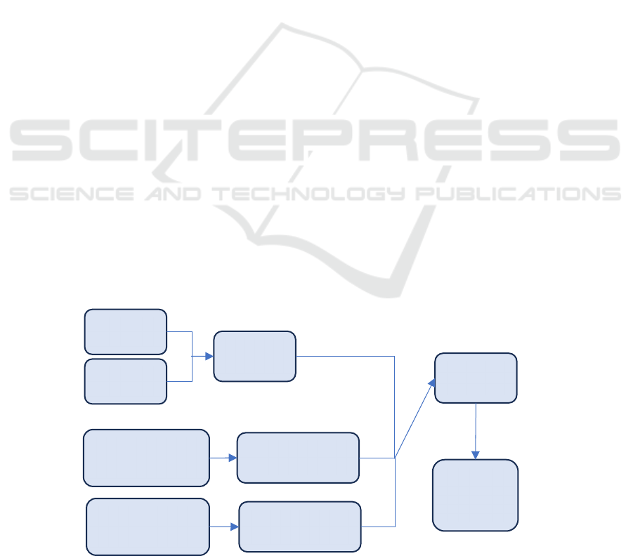
comprehensive process is illustrated in Figure 1

below.

2.2.1 MLP

One kind of feedforward neural network is the MLP.

The input layer, hidden layer, and output layer make

up an MLP. The hidden layer is represented by

learning features, the output layer generates the final

prediction, and the input layer receives the input data.

Each neuron of the hidden layer and the output layer

have activation functions which are used to introduce

nonlinear mapping. For the purpose of trying to

update the network parameters during training, the

error is backpropagated from the output layer back to

the input layer using the backpropagation technique,

which is required by MLP.

2.2.2 CNN

A popular deep learning model for computer vision

applications is CNN. CNN can handle image and

sequence data more efficiently than a standard neural

network because it can automatically identify

characteristics in images and extract relevant

information. Pooling layers, fully linked layers, and

convolutional layers make up CNN. CNN will

simultaneously apply certain regularizations to avoid

overfitting.

Convolution operation, which may determine an

image's sliding window and extract features through

filtering and pooling layers, is a fundamental

component of CNN. Convolution is a useful way to

minimize processing while maintaining the image's

spatial structural information. Pooling layers, without

altering the feature map's dimension, can lower

computation and increase the model's resilience.

2.2.3 Loss Function

When constructing MLP model and CNN model, the

Cross Entropy is used as the loss function. Cross

Entropy is often used in classification tasks, where it

can judge how close the actual and expected outputs

of a model are. The calculation formula is as follows:

𝐿𝑜𝑠𝑠  

∑

𝑥𝑙𝑜𝑔𝑥





(1)

The 𝑥 is the true label and the 𝑥 is the prediction label

output by the model. Since a picture corresponds to

only one label in general, there is only one 1 in the 𝑥

corresponding to a picture in the normalized label

data. For example, if 𝑥



1, 0, 0



, 𝑥

0.6, 0.3, 0.1, then the loss is calculated as follows:

𝐿𝑜𝑠𝑠  1×𝑙𝑜𝑔0.6  0×𝑙𝑜𝑔0.3  0×

𝑙𝑜𝑛𝑔0.1 𝑙𝑜𝑔0.6 (2)

2.3 Implementation Details

Some implementation details are explained below.

First of all, the task is done in Spyder (python 3.9),

and the training of the model is done on the GPU of

the personal computer. Secondly, the MLP model is

built by the torch framework, and the CNN model is

built by the keras framework. Thirdly, to draw an

image whose accuracy varies with the epoch, its

accuracy is recorded after each training session.

Thirdly, in order to draw images of the models’

changing accuracies, their accuracies are recorded

after each training epoch.

Figure 1: Overall process (Photo/Picture credit: Original).

MLP

CNN

Model

Structu

Three

Regularizations

Regularization

Four

Optimizers

Optimizer

Build

Model

Train

and

Predic

Image Discrimination and Parameter Analysis Based on Convolutional Neural Networks (CNN)

297

3 RESULTS AND DISCUSSION

This part compares and analyzes the models’ training

results. When constructing the model, the major

considerations are the effects of regularization,

optimizer, and model structure on accuracy. All three

affect the training and accuracy of the models.

3.1 Model Structure

After using the RMSprop and loss (cross entropy) to

build the models, the MLP model and the CNN

model are trained 100 epochs respectively. The

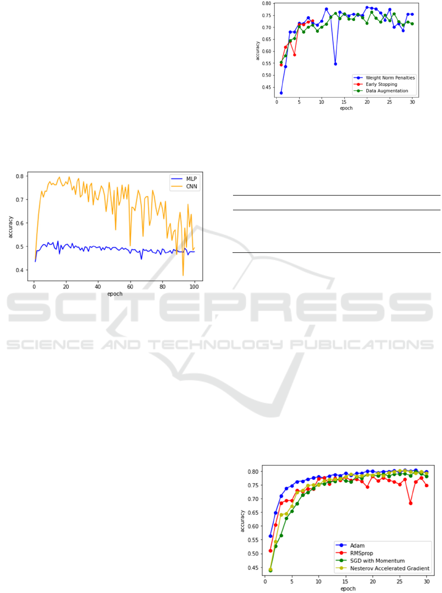
accuracies of the two models is shown in Figure 2.

Figure 2: Accuracies of the two models (Photo/Picture

credit: Original).

The Figure 2 illustrates that the accuracy of the

CNN model varies in a large range, while the

accuracy of the MLP model has been maintained in a

small interval. From the highest accuracy achieved

by the models, the CNN’s is 79.54%, while the

MLP’s is 52.13%. There is a large difference between

the two accuracies, which indicates that the model

structure has a significant impact on the training

results. It can be seen from the comparison that CNN

has more advantages, so the CNN model is chosen in

the subsequent trainings.

3.2 Regularization

From the above results, it can be seen that the model

has reached the optimal accuracy when the epoch is

22. For more efficient training, the following

trainings use 30 epoch. After the models are

constructed and trained, the accuracy variation

graphs of weight norm penalties (WNP), early

stopping (ES) and data augmentation (DA) can be

obtained in Figure 3.

WNP has the highest accuracy of 78.36%. The

highest accuracies of the three regularizations and

Figure 3: Accuracy variations of three regularizations

(Photo/Picture credit: Original).

the corresponding epoch are shown in the following

table.

Table 1: Accuracies and epoch of three regularizations.

ularizations Accurac

och

WNP 78.36% 20

ES 72.85% 8

DA 76.33% 21

As shown in the Table 1, WNP is a regularization

method with weights, which can effectively constrain

the size of models’ parameters and control models’

complexity. WNP can also facilitate the model to

learn more generalized feature representations, which

improve the model's performance in image

classification tasks. Remarkably, although WNP has

the highest accuracy, ES achieves a high accuracy

after 8 training stops. This can make the model

training more convenient and faster.

3.3 Optimizer

Four optimizers, Adam, RMSprop, SGD and

nesterov accelerated gradient (NAG), are used to

build and train the models. The accuracy variations

are shown in the Figure 4.

Figure 4: Accuracy variations of four optimizers

(Photo/Picture credit: Original).

EMITI 2024 - International Conference on Engineering Management, Information Technology and Intelligence

298

The model constructed by Adam has the highest

accuracy of 80.27%. The highest accuracies reached

by the four optimizers and the corresponding epoch

are shown in the Table 2.

Table 2: Accuracies and epoch of four optimizers.

ularizations Accurac

och

Adam 80.27% 28

RMSprop 78.09% 20

SGD 79.76% 28

NAG 80.11% 25

Adam includes an adjustable learning rate

function that allows it to dynamically modify the

learning rate during training in order to accommodate

various parameter characteristics.

3.4 Final Model

After the model structure, regularization, and

optimizer are selected, the final model can be built.

The parameters and accuracy of the final CNN model

are shown in the Table 3.

Table 3: Parameters and accuracy of final model.

ularization O

timize

och Accurac

WNP Adam 28 79.86%

Following model training, classification

predictions can be produced. A few of the anticipated

outcomes are displayed in Figure 5.

Figure 5: Classification prediction results (Photo/Picture

credit: Original).

It can be seen that the classification effect of the

model is good, and most objects can be correctly

classified. But some objects with ambiguous features

can be misjudged. It should be pointed out that due to

the randomness of machine learning, the final

model's correctness is different from the accuracy in

the selection process.

4 CONCLUSION

This study sheds light on the impact of model

structure, regularization techniques, and optimizers

on accuracy, aiming to pinpoint the optimal

parameter combination for the final model.

Employing two distinct model structures, three

regularization methods, and four optimizers, we

conducted a comprehensive analysis of each

variable's influence. At each stage, a singular

parameter was manipulated to construct various

models, with subsequent comparison of their

performance through accuracy change visualization.

This approach enabled us to discern the influence of

each parameter and identify the optimal parameter

combination. Our findings indicate that the CNN

model outperforms the MLP model in Cifar-10 image

classification tasks, with WNP demonstrating the

most favorable effect among the three regularization

methods, and Adam emerging as the top-performing

optimizer among the four options. Notably, the

efficacy of various parameters varies across different

deep learning tasks, underscoring the need for careful

consideration of theoretical and empirical factors

when determining the optimal parameter

combination. Furthermore, it is crucial to recognize

that optimal accuracy does not necessarily equate to

the optimal model, as factors such as data structure,

training cost, and task requirements must be

comprehensively evaluated. Looking ahead, future

research endeavors will explore the influence of

additional parameters on model performance, with a

focus on identifying optimal parameter combinations

for advanced models that excel in image

classification tasks.

REFERENCES

Karpathy, A. (2017). Convolutional neural networks for

visual recognition. Notes accompany the Stanford CS

class CS231.

Hossain, M. A., & Sajib, M. S. A. (2019). Classification of

image using convolutional neural network (CNN).

Image Discrimination and Parameter Analysis Based on Convolutional Neural Networks (CNN)

299

Global Journal of Computer Science and Technology,

19(D2), 13-18.

Goodfellow, I., Warde-Farley, D., Mirza, M., Courville, A.,

& Bengio, Y. (2013, May). Maxout networks. In

International conference on machine learning, 1319-

1327, PMLR.

Stollenga, M. F., Masci, J., Gomez, F., & Schmidhuber, J.

(2014). Deep networks with internal selective attention

through feedback connections. Advances in neural

information processing systems, 27.

Liang, M., & Hu, X. (2015). Recurrent convolutional

neural network for object recognition. In Proceedings

of the IEEE conference on computer vision and pattern

recognition, 3367-3375.

Huang, G., Liu, Z., Van Der Maaten, L., & Weinberger, K.

Q. (2017). Densely connected convolutional networks.

In Proceedings of the IEEE conference on computer

vision and pattern recognition, 4700-4708.

Liang S, Khoo Y, Yang H. Drop-activation: implicit

parameter reduction and harmonious regularization.

Communications on Applied Mathematics and

Computation, 2021, 3, 293-311.

Lu, D., & Weng, Q. (2007). A survey of image

classification methods and techniques for improving

classification performance. International journal of

Remote sensing, 28(5), 823-870.

Nazir, S., Patel, S., & Patel, D. (2018, July). Hyper

parameters selection for image classification in

convolutional neural networks. In 2018 IEEE 17th

International Conference on Cognitive Informatics &

Cognitive Computing (ICCI* CC), 401-407, IEEE.

Bera, S., & Shrivastava, V. K. (2020). Analysis of various

optimizers on deep convolutional neural network

model in the application of hyperspectral remote

sensing image classification. International Journal of

Remote Sensing, 41(7), 2664-2683.

Krizhevsky, A., & Hinton, G. (2009). Learning multiple

layers of features from tiny images, University of

Toronto, 7.

EMITI 2024 - International Conference on Engineering Management, Information Technology and Intelligence

300