Creation of Training Data and Training for Prediction Model of Curling

Scores Using Real Game Data

Tomoya Iwasaki

, Wataru Noguchi

2 a

, Yasumasa Tamura

3 b

, Shimpei Aihara

4 c

and Masahito Yamamoto

3 d

Graduate School of Information Science and Technology, Hokkaido University, Hokkaido, Japan

Education and Research Center for Mathematical and Data Science, Hokkaido University, Hokkaido, Japan

Faculty of Information Science and Technology, Hokkaido University, Hokkaido, Japan

Department of Sport Science and Research, Japan Institute of Sport Sciences, Tokyo, Japan

Keywords:

Curling, Digital Curling, Curling AI, Expectimax, Evaluation Function, Wining Probability, Game Tree

Search, Results Book.

Abstract:

Curling is a sport in which two teams take turns shoting stones at each other on an ice ﬁeld to compete for

total scores. Curling is a highly strategic sport, and the strategy of stone delivering has a signiﬁcant impact on

the outcome of the game. To verify strategy of curling, “digital curling” is a platform that reproduces curling

on a computer. Following the previous research of curling AI using game tree search and evaluation function

by Ataka et al., real game data was obtained and trained into a neural network of evaluation function. In this

study, we propose a method to obtain stone position information from real game data. Also, the model was

trained from the obtained data. The results show that models trained with realistic data correspond better to

realistic situations than conventional models trained with data generated by algorithms. However, in situations

where there are many stones on the sheet, the model was also found to be insufﬁciently accurate as is the case

with conventional models.

1 INTRODUCTION

Curling is a sport played on a ﬁeld of ice, in which

two teams take turns delivering stones and compete

for the ﬁnal total score. In curling, not only the skill

of delivering the stones to the target position, but also

the strategy of where and how to deliver the stones has

a great inﬂuence on the game result. Because of this

highly strategic aspect, curling is also called “Chess

on Ice”.

To evaluate curling strategy, a computational sim-

ulation platform called digital curling has been uti-

lized recently. The digital curling platform enables

AI-based curling players to play against each other

(Uehara and Ito, 2021). The strategies veriﬁed by this

simulator are expected to be applicable to real curling,

and curling AI researches are active on this platform.

Various approaches have been attempted to study

curling AI by digital curling. Among them, Ya-

mamoto et al. discretize the the ﬁeld (called “sheet” in

https://orcid.org/0000-0002-0250-4128

https://orcid.org/0000-0001-5406-1966

https://orcid.org/0000-0002-8513-0204

https://orcid.org/0000-0002-7326-3691

curling) into a grid and use the game tree search (Ya-

mamoto et al., 2015). And Katoh et al. use the Expec-

timax search algorithm to perform game tree search in

curling with uncertainty (Katoh et al., 2016). These

studies have shown that the search for candidate shots

in continuous and uncertain curling games is possible

with game trees. In addition, Yamamoto et al. de-

velop a neural network based state evaluation function

and showed that it is more effective than hand-crafted

evaluation function (Yamamoto et al., 2018). Further-

more, Ataka et al. added the game situation to the

input of the neural network to allows score prediction

based on the game situation such as score difference

(Ataka et al., 2020).

In this study, we aimed to utilize game data from

actual curling competitions for training a score pre-

diction model. In previous research used data auto-

matically generated based on algorithms or obtained

from self-competitions between curling AIs for train-

ing data. However, such automatically generated data

may be inadequate as training data in that it is far from

the actual game phase and lacks diversity. Therefore,

we aimed to utilize game data from actual curling

competitions to train a score prediction model capable

of responding to various realistic situations. In the ex-

168

Iwasaki, T., Noguchi, W., Tamura, Y., Aihara, S. and Yamamoto, M.

Creation of Training Data and Training for Prediction Model of Curling Scores Using Real Game Data.

DOI: 10.5220/0012941100003828

Paper published under CC license (CC BY-NC-ND 4.0)

In Proceedings of the 12th International Conference on Sport Sciences Research and Technology Support (icSPORTS 2024), pages 168-179

ISBN: 978-989-758-719-1; ISSN: 2184-3201

periment, we collected two sets of training data, one

from actual game data and one from algorithms used

in previous research, and compared the performance

difference due to the difference of training data.

2 CURLING

Curling is played on a ﬁeld of ice called a “sheet”. An

overview of the sheet is shown in Fig. 1. Sheet has a

circular area called a “house” and kickstand called a

“hack”. Delivering a stone from hack side to the op-

posite house side is called a “shot”. Both teams shoot

stones in an attempt to leave more stones in the house.

When shoting, the player must release his or her hand

from the stone before reaching the “hog line” on the

hack side. The stones are active if they remain station-

ary between the hog line and back line on the house

side. Otherwise, the stones are regarded as invalid and

removed from the sheet. The sheet can be swept with

a broom after the stone has been shot. This allows the

trajectory of the stone to be adjusted.

An inning in a game is called an “end”, and a

game usually consists of eight or ten ends. The team

with the highest total score at the end of ﬁnal end

wins. If both teams are tied, the game continues in

extra ends until one of teams wins a score difference.

It is also possible to resign the game in the middle of

the game, which is called “concede”.

In each end, both teams take turns shoting eight

stones. An end ends when the second team shots the

last stone. This last stone is called the “hammer”. To

allow more stones to be stored on the sheet, the “free

guard zone rule” exists. This rule prohibits the stones

in the free guard zone (area between hog line and tee

line, excluding house) from leaving the playing area

until the ﬁfth shot of overall is completed. It is pos-

sible to move stones slightly as long as they are not

moved out of the playing area. If this rule is violated,

the shot stone will be removed and the moved stone

will be returned to its original position. At the end of

an end, only the team with the stone closest to the

center of the house among the stones in the house

gains scores. Scores are awarded for the number of

stones inside the house that are closer to the center

of the house than the opposing team’s closest stone.

The team that awarded scores takes the ﬁrst shot in

the next end. If there is no stone inside the house,

no scores are awarded to either team. This is called

a “blank end,” and the ﬁrst team in a blank end plays

ﬁrst in the next end. In other words, the playing order

switches if either team gains one or more score in the

previous end.

As mentioned above, in curling, the score is de-

termined when the last shot of the second offensive

team is completed. In this sense, curling is a sport

in which the second team has an overwhelming ad-

vantage. Therefore, it is necessary to adopt different

strategy for the ﬁrst and second offensive teams. Gen-

erally, the ﬁrst team aims to let the second team to

score one point, so that the team will get the hammer

in the next end. Alternatively, the ﬁrst team aims to

gain scores instead of the second team called “steel”.

The second team, on the contrary, aims to score two

or more points or, to maintain hammer by removing

all stones from the house to make it a blank end. Both

teams proceed with the game, constructing strategy

to achieve the desired stone position for their team at

the end of the end. Each team must decide on their

strategy and shot stone within the allotted time limit.

Figure 1: Overview of the sheet. The player shots a stone

in the direction of the opposite house from the hack. The

distance from the hack to the hog line on the hack side is 33

feet. The distance to the opposite hog line is 105 feet, to the

tee line is 126 feet, and to the back line is 132 feet.

3 DIGITAL CURLING

Digital curling is a platform for reproducing curling

on a computer. Digital curling enables curling AIs to

play against each other. Games in digital curling are

conducted through communication between the digi-

tal curling simulator and each AI. The simulation is

performed by a physics engine. The game is played

according to the rules of real curling.

The curling AI sends shot information to the digi-

tal curling simulator, which simulates the shot and re-

turns the result to the AI. The AI sends shot informa-

tion, including the 2-dimensional vector and direction

of rotation, to the simulator. Then the simulator runs a

simulation based on the current game information and

the input shot information, and sends the results to

each AI. The information from the simulator includes

the position of each stone, the current score, and the

team that will play the next shot. The positions of the

stones are represented by a two-dimensional coordi-

nate system. Simulations are performed at discretized

regular intervals by a physics engine that calculate tra-

jectories and collision detection. The results of the

simulation can be viewed on the GUI as shown in Fig.

The number of ends and AI thinking time can be

Creation of Training Data and Training for Prediction Model of Curling Scores Using Real Game Data

169

set arbitrarily. The presence or absence of the free

guard zone rule can also be set. These settings are

disclosed in advance in curling AI competitions using

Digital curling.

In real curling, due to the inﬂuence of sheet con-

ditions and the skill of the players, it is not always

possible to place the stones precisely at the target po-

sition. In real curling game, this uncertainty must be

taken into account when making strategic decisions.

To reproduce this, a random ﬂuctuation is added to a

given shot vector in digital curling. The setting about

the scale of random ﬂuctuation can be set for each

player. In competitions, the setting is disclosed.

Figure 2: Simulation result on GUI. The trajectories and re-

sults of all shots during a digital curling game can be viewed

on GUI.

4 CURLING AI IN DIGITAL

CURLING

Previous research (Katoh et al., 2016) has shown that

game tree search and evaluation functions can be used

to build an AI that is superior to a curling AI built on

rule based methods. In this study, we construct an

evaluation function with reference to the curling AI

of Ataka et al. The evaluation function consists of

an expected score distribution and a winning proba-

bility table. The expected score distribution is calcu-

lated from the game situation using a score prediction

model.

The score prediction model needs to be trained

with curling game information such as stone posi-

tions. In the previous research, the model was trained

by data generated by the algorithm. On the other

hand, in this study, we aim to utilize data from real

curling competitions in order to make the Curling AI

to adapt diverse and realistic situations.

4.1 Search in Digital Curling

The evaluation function maps a given game situation

to a quantitative value. Ataka et al. have shown that

the expected winning probability can be used as the

evaluation value, allowing evaluation according to the

situation of the curling game. The evaluation function

consists of a score prediction model and a winning

probability table.

The expected score distribution is the probability

distribution of the score obtained at the end of an end.

In digital curling, the score obtained at the end of an

end is uncertain because of the uncertainty involved

in the shot. Also, in curling, the winning probabil-

ity signiﬁcantly depends on the number of scores ob-

tained. Therefore, the distribution of expected score

is used instead of simply relying on the value of ex-

pected score.

A winning probability table is a table showing a

team’s winning probability based on the number of

remaining ends in a game and the difference in to-

tal score to the opponent team. In curling, the opti-

mal strategy can vary greatly based on the number of

remaining ends and the score difference. In particu-

lar, maximizing the number of scores for a single end

does not always lead to maximizing the winning prob-

ability, because the blank end is an effective strategy

for the team having hammmer. The winning proba-

bility table makes it possible to deal with such situ-

ations. By combining the winning probability table

and the expected score distribution, the expected win-

ning probability at the end of that end can be com-

puted. Table. 1 shows the winning probability table

used in this study. It was obtained by self-competition

between curling AIs in previous research and shows

the winning probability of the ﬁrst team in each situ-

ation.

Table 1: Winnig probability table to be used. The table

shows the winning probability of the ﬁrst team for each

score difference and the number of remaining ends.

remaining ends

3 2 1 0

Difference of score

3 0.919 0.946 0.962 1.000

2 0.771 0.794 0.881 1.000

1 0.609 0.557 0.677 1.000

0 0.340 0.279 0.260 0.220

-1 0.162 0.122 0.042 0.000

-2 0.034 0.021 0.011 0.000

-3 0.015 0.014 0.011 0.000

icSPORTS 2024 - 12th International Conference on Sport Sciences Research and Technology Support

170

4.2 Score Prediction Model

The score prediction model computes the expected

score distribution at the end of an end based on the

game situation without simulating all possible shots

until the end of the end. The model is constructed

by a simple fully-connected neural network. As input

data for the model, positioning information of stones

on the sheet and information of the game situation are

used. The information for each stone, as shown in

Table2, is inputted in order of proximity to the cen-

ter of the house for all ﬁfteen stones. Information of

stones that do not exist on the sheet are all set to 0.

Information of the game shown in Table3 is also in-

put to the model. These are all one-hot vectors. The

output of the model is an 11-dimensional distribution

of expected scores. This indicates the probability of

scoring from -5 to 5 scores at the end of end. The

activation function of the output layer uses softmax.

Table 2: List of information of stones. Coordinates and dis-

tance from the center of house are represented as continuous

values, while other data are represented as discrete values.

Information Value

x coordinate [-2.375, 2.375]

y coordinate [32.004, 40.234]

Distance from center of house [0, 6.78]

Is there stone in the play area 0, 1

Is there stone in the house 0, 1

Owned player -1, 0, 1

Is there enemy stone on the inside 0, 1

Table 3: List of information of game. These information are

input in one-hot vectors.

Information Value(one-hot vector)

Score difference -2,-1,0,1,2

Remaining ends 0,1,2,3

4.3 Creation of Training Data

In this study, training data was created only for the

last shot of the end. Because the score of the end is

determined when the last shot is completed, so multi-

ple stages of simulation are not necessary, and the ex-

pected score distribution can be obtained with a small

number of simulations.

First, the number of remaining ends, score differ-

ence, and stone position data are given as input data

for the model. In this situation, all candidate shots

are simulated on the digital curling. Each candidate

shot is a vector of shots that reach each score on the

sheet divided on the grid. Grid is a square and its size

is the radius of the stone. No random ﬂuctuation are

added to the simulation at this time. The score is cal-

culated from the stone position obtained after simula-

tion. Based on the points scored, the score difference

in the game situation and the number of remaining

ends, the expected winning probability is calculated

using the winning probability table. The formula for

this calculation is shown in Eq. 1.

E(x, y) =

∑

∆x=−3

∑

∆y=−5

p(x

, y

)w(r, d, s(x

, y

)) (1)

where x

= x + ∆x, y

= y + ∆y

p(x

, y

) is the probability of the shot stone reach-

ing the grid around the candidate shot after the simu-

lation when a random ﬂuctuation is added to the can-

didate shot. ∆x and ∆y are the deviations from the grid

of the candidate shot. We consider 3 grids in the x di-

rection and 5 grids in the y direction centered on the

grid of the candidate shot. Since the random ﬂuctu-

ation added to the shot are predetermined, the proba-

bility of the stones reaching the surrounding grids can

be determined in advance. w(r, d, s) is the expected

winning probability when the ﬂuctuation of remain-

ing ends r, the score difference d, and the score at the

end of the end is s. This can be obtained from Table.

1. s(x

, y

) is the score at the end of the end when a

shot is made at x

and y

, obtained from the simulation

without random ﬂuctuation described above.

Thus, we obtain the expected winning probability

for all candidate shots. The candidate shot with the

highest expected winning probability obtained is con-

sidered the best shot. Finally, we simulate this best

shot multiple times with the original stone arrange-

ment. Since random ﬂuctuations are added to this

simulation, a probability distribution for each score

can be obtained. This probability distribution is the

expected score distribution as the target output, corre-

sponding to the game situation as the input.

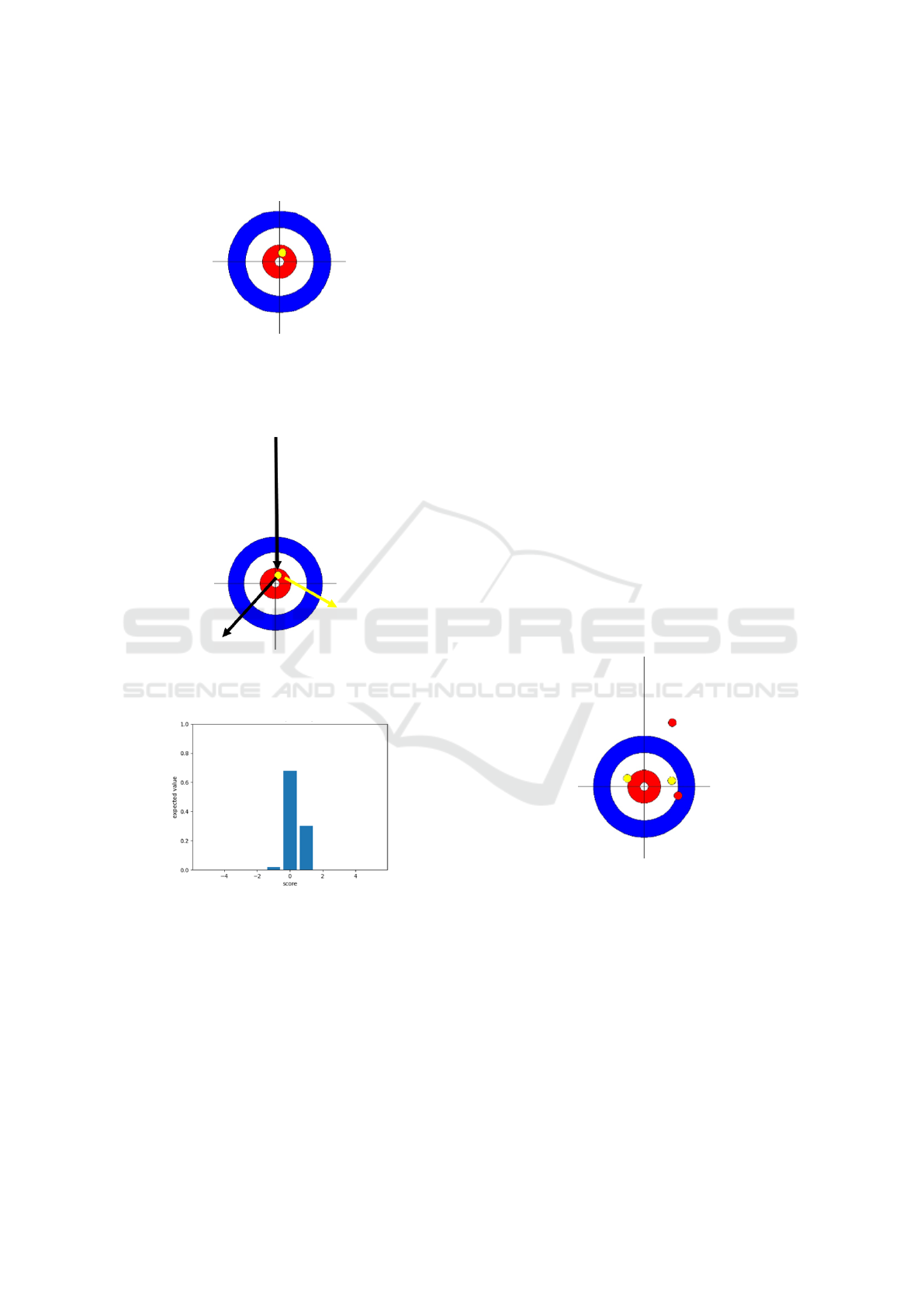
As an example, the number of remaining ends is 1,

the score difference is 0, and the stone position is the

data shown in Fig. 3. Table. 1 shows that the winning

probability in this situation is about 67% if one point

is gained, 74% if a blank end is assumed, and about

4% if one point is lost. In other words, blank end

and scoring one point are high winning probability

actions, with blank end having the highest value. In

the situation, a shot as shown in the Fig. 4 is the best

shot in this situation because the expected winning

probability according to Eq. 1 is the highest. After

simulating the best shot multiple times, the expected

score distribution is as shown in Fig. 5. Fig. 5 shows

an example situation that can be blank end about 80%

of the time, but it is also a situation that a single point

be scored . It also shows that there is almost no risk

of steal. This means that the best shot in this situation

Creation of Training Data and Training for Prediction Model of Curling Scores Using Real Game Data

171

will succeed 80% of the time, and even if it fails, there

is little possibility of steal.

Figure 3: Example of stone position. There is only one

stone of the opposing team near the center of the house.

The situation of the game is that the number of remaining

ends is one, the score difference is 0, and the next shot is

the last shot of the end.

Figure 4: Example of shot. The black arrows are the shot

stone trajectories. The yellow arrow is the trajectories of

stones that move in collision with the shot stone.

Figure 5: Expected score distribution in the example. The

expected score distribution indicates that this situation is al-

most risk-free, but the success of the best shot (blank end)

is not assured.

4.4 Example of Training Data

By creating training data using the method described

in the previous section, it is possible to create training

data that corresponds to the situation in which strate-

gies change signiﬁcantly depending on the game situ-

ation.

First, let us assume that the common situation is

that the team has the red stone, next shot is the last

shot and the stone position as shown in Fig. 6, With

this stone position, it is easy for a red team to score

one point by simply placing a stone in the center of the

house, but relatively difﬁcult for a team to score two

points because it requires double takeout of the yellow

stones. Blank end is almost impossible because team

need to take out all three stones in the house and the

shot stone must not be left in the house. On this case,

the ﬁrst situation is set with a score difference of 0,

end 9th, and the second situation is set with a score

difference of -2, end 10th.

In the ﬁrst situation, the team should try to score

one point safely, because if the team is stolen points,

winning probability will signiﬁcantly decrease. In the

second situation, the team must attempt to score two

points, even though there is a high risk, because if

two points are not scored, the game is lost at that

point. The expected score distributions obtained by

the method in the previous section are shown in Fig.

7 for the ﬁrst situation and in Fig. 8 for the second

situation. The ﬁrst situation shows that one point can

be obtained reliably. The second situation shows that

the success rate is low, but two points can be obtained.

Thus, the expected score distribution in training data

can take into account situations where high risk/high

return is required and situation where low risk/low re-

turn is required.

Figure 6: Position before last shot. The opposing team has

the No. 1 and No. 2 stones and own team has the No. 3

stone.

5 TRANING DATA EXTRACTION

FROM REAL CURLING GAMES

The data information required to compose the training

data are stone position, score difference, and number

of remaining ends. We obtain stone placement data

from real games, instead of utilizing data extracted

from self-playing by AI-based players or automati-

cally generated based on algorithms.

icSPORTS 2024 - 12th International Conference on Sport Sciences Research and Technology Support

172

Figure 7: Expected score distribution for situation required

low risk strategy. The distribution shows that the best shot

is sure to succeed.

Figure 8: Expected score distribution for situation required

high risk strategy. The distribution indicates that the best

shot is the shot with the greatest risk.

5.1 Results Book

Game data was obtained from the “Results Book”

provided by Curlit, a PDF ﬁle containing informa-

tion on major curling competition in the world (Curlit,

2024). The Results Book contains pages called “Shot

by Shot”, which show the sheet information including

the location of the stones in each shot, shown in the

image (Fig. 9) (Curlit, 2022) . The coordinates of the

stones are obtained from these images.

5.2 Data Extraction from Results Book

We extract three types of data: the stone positions,

the ﬁrst shot team in the corresponding end, and the

shot number. These data are stored in the database.

An existing work (Myslik, 2020) provided a method

to extract those data from the earlier version of Result

Books. Based on Myslik’s work, we implemented an

enhanced script compatible with the latest version of

Result Books.

Data extraction is done as following. First, we

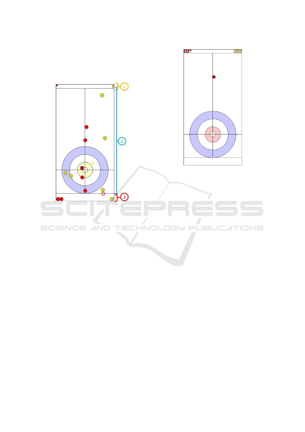
split the Results Book by game. An image is taken

from the shot by shot page showing stone position in

shot order. The image obtained at this time is shown

in Fig. 10. This image shows the number of stones

remaining for each team, stones existing on the sheet,

Figure 9: Example of Shot by Shot. The stone positions of

the sheets are listed as images in the order of the shots.

stones moved by the previous shot (represented by

colored frames only) , and stones removed from the

game. From this image, only the stones on the sheet

necessary for the training data are extracted.

The ﬁrst shot team is determined from the ﬁrst

shot image as shown in the Fig. 11. Since the ﬁrst

image shows the sheet after the ﬁrst team has already

made a shot, the number of stones remaining for the

ﬁrst team is seven. Therefore, the team with lower

number of stones remaining is the ﬁrst team.

Next, the contour information of the area having

the same color as the stones is obtained from the im-

age. However, areas other than stones on the sheet

may be unintentionally included in the resulting con-

tours. Therefore, it is necessary to exclude extra con-

tour information. First, the color of the center of the

contour is obtained and those that do not have the

same color as the stones are excluded. The stones

moved by the previous shot can be excluded by this

requirement since they are represented only by a col-

ored frame. Next, contours that are too large or too

small are excluded. Since the stones on the sheet are

shown at approximately the same size, it is possible

to exclude contour information obtained incorrectly.

Finally, contours whose center coordinates are not on

the sheet are excluded. This allows for the removal

Creation of Training Data and Training for Prediction Model of Curling Scores Using Real Game Data

173

of stones that are unrelated to the game, located at the

top and bottom of the sheet image. The coordinates

of the remaining areas, which are determined as the

stones, are converted to the coordinate system of dig-

ital curling and stored in database.

Figure 10: Image showing stones on sheet obtained from

Shot by Shot. Area 1 shows the number of stones before

the shot for both teams. Area 2 shows the position of the

stones on the sheet and various information representing the

progress of the game. Area 3 shows the number of stones

from both teams already removed from the game.

5.3 Data Extraction Results

In this work, game data was obtained from the Re-

sults Book of eight competitions after the “No tick

rule” was applied. The competitions used were Eu-

ropean curling Championships 2022, European curl-

ing Championships 2023, Pan Continental curling

Championships 2022, Pan Continental curling Cham-

pionships 2023, World Junior curling Championships

2022, World Junior curling Championships 2023,

World Women’s curling Championships 2022 and

World Men’s curling Championships 2022. In total,

we were able to obtain data for 532 competitions with

74,857 games. The number of data extracted per shot

is shown in Table 4. More than 4600 data were ex-

tracted for each shot.

A comparison of the original image and the ex-

tracted data illustrated in the coordinate system of

digital curling is shown in Fig. 12. In Fig. 12, the

positions of stones are almost the same as the origi-

nal image in the coordinate system of digital curling.

This shows that this method can obtain accurate stone

Figure 11: Sheet image after the ﬁrst shot. This is the ﬁrst

sheet image on the page for each end. In this case, the red

team made the ﬁrst shot, so there is one less red stone re-

maining at the top of the image.

position data even when there are many stones and

other information on the sheet.

Fig. 13 compares the distribution of the number

of stones each team holds: the number of ﬁrst team’s

stones on x-axis, and that of second team’s stones

on y-axis. According to Fig. 13, the data extracted

from Results Book (on the right) obviously contains

more situations with considerably many stones than

the data generated by the algorithm (on the left). Also,

the ﬁrst team tends to hold more stones than the sec-

ond team in the data extracted from Results Book.

This comparison shows that the data extracted from

Results Book includes diverse realistic situations.

5.4 Creation of Training Data from

Extracted Data

Following the procedure outlined in Section 4.3, we

created the training data to be used in training from

the game information extracted in the previous sec-

tion. The training data consists of pairs of game infor-

mation, including extracted stone positions, remain-

ing ends, and score difference, along with the corre-

sponding expected score distribution.

Below, we evaluate the quality of the created data.

By comparing the actual game results with the ex-

pected score distribution generated by the method in

Section 4.3, we will conﬁrm that the training data is

somewhat realistic, i.e., not unnatural compared to the

actual player’s strategy.

icSPORTS 2024 - 12th International Conference on Sport Sciences Research and Technology Support

174

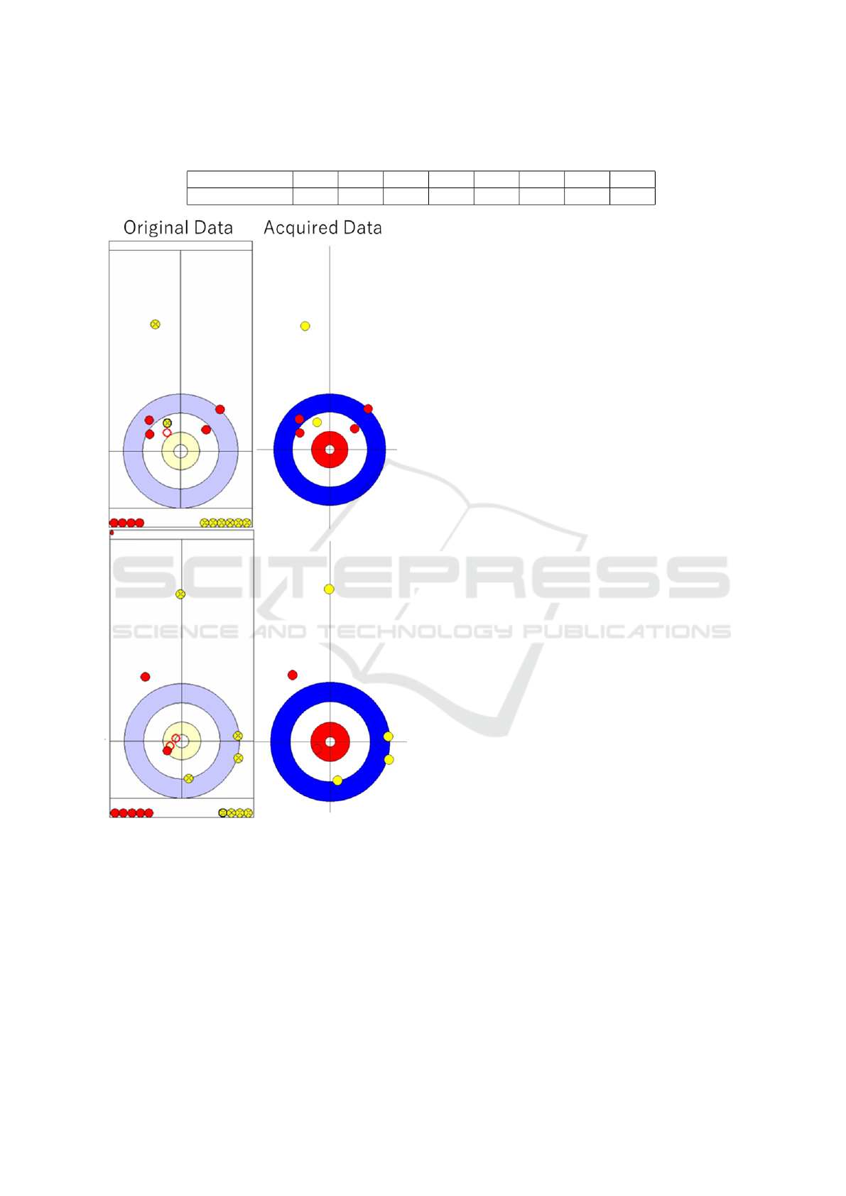
Table 4: Number of data per shot. About 4600 data were obtained per each shot. The reason for the smaller number of data

in the late game is that the game may end before last end due to concede.

Shot number 1-9 10 11 12 13 14 15 16

Number of data 4690 4687 4684 4682 4663 4663 4650 4590

Figure 12: Comparison of extracted data with the original

image. The original image is on the left and the extracted

data is illustrated again by coordinate of digital curling on

the right.

The game information used is from World

Women’s curling Championships 2022. The situation

is that the team is the yellow stone, score difference

of -2 and the last shot in the 7th end. The stone po-

sitions is as shown in Fig. 14. The expected score

distribution in this situation is shown in Fig. 16. In

the actual game, the team’s shot was successful, the

stone position was as shown in Fig. 15, and the team

scored three points. From Fig. 16, in the expected

score distribution we created, the probability of ob-

taining three points is nearly 80%. In other words,

it was shown that it is possible to obtain an expected

score distribution in line with real players’ strategies

as training data for the model from the positions of

stones in actual games.

6 MODEL TRAINING AND

RESULTS

The obtained training data will be used to train and

validate the score prediction model. Validation is per-

formed by comparing models trained by real data with

models trained by data generated by conventional al-

gorithms.

6.1 Training Model

The number of stone positions used to train the model

is 4650 for both real and generated data. For each

of these stone positions, there are 5 different cases

in terms of score difference and 4 cases in terms of

the number of remaining ends, so the training data is

93,000. The x-coordinates of the stone position were

inverted to increase the number of data, since the ef-

fect of inversion on the x-coordinates is negligible.

The ﬁnal number of training data is 186,000. One

hundred out of 4650 stone positions were used as val-

idation data. This means that the model has 182,000

training data and 4,000 validation data.

The model has three hidden layers, each with 200

neurons. The activation function of the hidden layer

uses ReLU. The hidden layer includes batch nor-

malization and dropout. The optimization function

used during training was Adam, the learning rate was

0.001, the batch size was 1024, the dropout rate was

0.3, and the loss function was the mean squared error.

The training was conducted for 100 epochs with these

parameters. The loss during training was as shown in

Fig. 17. Mean squared error is used for the loss func-

tion. The training and test loss are decreasing, but the

test loss is higher.

6.2 Results

We validated whether the trained models could pre-

dict accurate expected score distribution in multiple

Creation of Training Data and Training for Prediction Model of Curling Scores Using Real Game Data

175

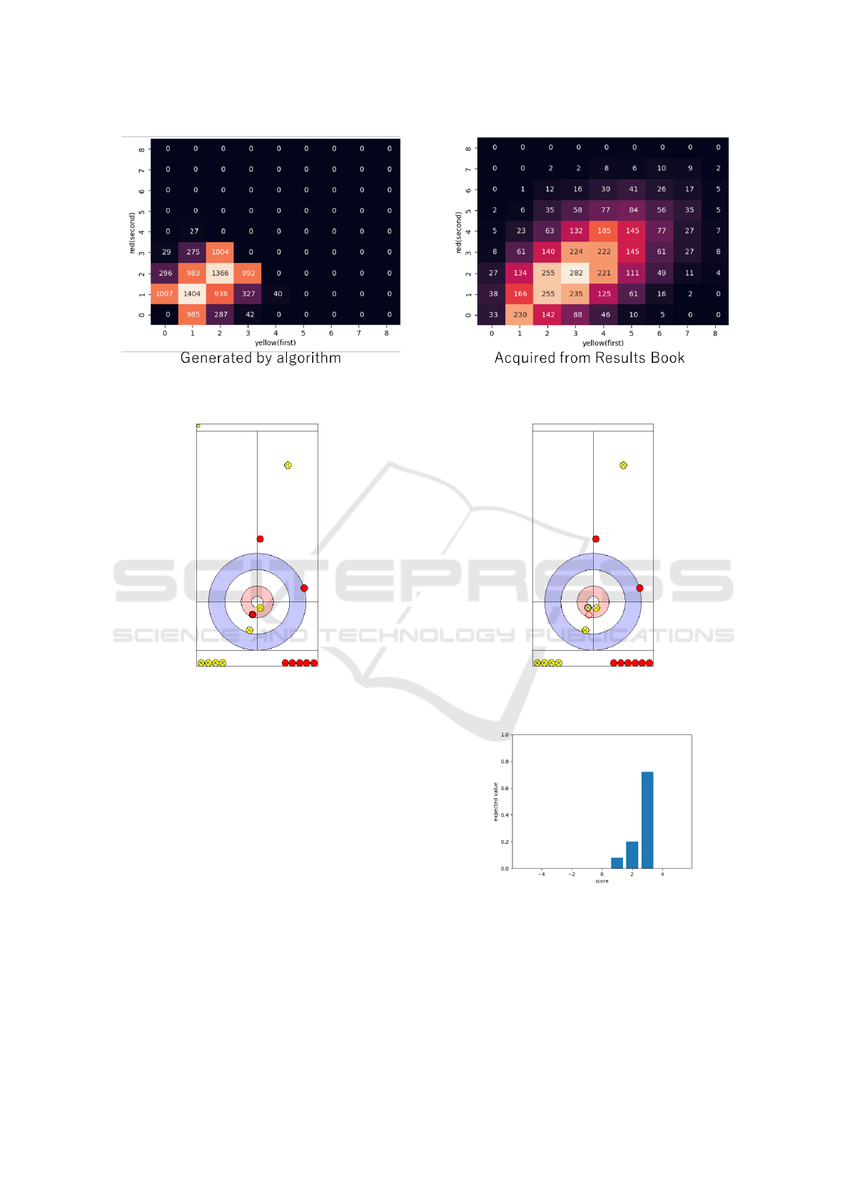
Figure 13: Distribution of number of stones for each team in train data. In each ﬁgure, the horizontal axis shows the number

of stones for the ﬁrst team and the vertical axis shows the number of stones for the second team.

Figure 14: Position before last shot. Own team (yellow

stone) has the No. 1 stone, but own team must take out

the opposing team’s No. 2 stone in order to obtain multiple

scores.

situations. In which ﬁgure of stone positions in each

situation, the stones of the own team are shown in red

and those of the opposing team in yellow. The pre-

diction results for these situations are show in Fig.

18, 19 and 20. In the ﬁgure, from left to right, the

correct score distribution, the prediction results from

the real model, and the prediction results from the

conventional model. The correct score distribution is

the expected score distribution created according to

the training data creation method described in Section

4.3.

Situation 1 is a situation in which the stone po-

sition is Fig. 18, the score difference is 0, and the

number of remaining ends is 0. The stone position in

Fig. 18 is a simple situation with a small number of

stones. The prediction result in this case is shown in

Fig. 18. In this situation, the team can win the game

Figure 15: Stone position after Fig. 14 shot in the actual

competition. The shot was successful and own team scored

3 points.

Figure 16: Expected score distribution created from the sit-

uation. The probability of three scores, which is the score

obtained in the actual game, is nearly 80%. This result is in

line with the actual strategy of the players.

if team’s stone becomes the No. 1 stone, so the team

have to take out the opponent’s stone in the house and

leave shot stone in the house. Since this shot is of low

difﬁculty, the correct score distribution shows that a

icSPORTS 2024 - 12th International Conference on Sport Sciences Research and Technology Support

176

Figure 17: The learning curve. Mean squared error is used

for the loss function. The orange curve is for validation data

and the blue curve is for train data.

point will almost certainly be scored. In this case,

both models are accurate in their predictions.

Situation 2 is a situation in which the stone po-

sition is Fig. 19, the score difference is -1, and the

number of remaining ends is 0. The stone position

in Fig. 19 is more complicated than situation 1 be-

cause there are more stones. In this situation, the team

can win the game by scoring 2 points, so it is neces-

sary to leave the shot stone in the house while tak-

ing out the opposing team’s stones without touching

the our team’s stones in the house. Since this shot

is a highly difﬁcult shot, the correct score distribu-

tion shows that although there is a high possibility

of gaining two points, there is a risk of gaining only

one point or, even loosing the game by being steeled

by the opponent. From Fig. 19, we can see that the

model learned with real data is able to predict the sim-

ilar distribution as the correct score distribution. On

the other hand, the conventional model has the high-

est probability of gaining 2 points, but there is also a

probability of gaining 3 points, which is impossible,

indicating that the conventional model does not accu-

rately understand the situation in prediction.

Situation 3 is a situation in which the stone po-

sition is Fig. 20, the score difference is 0, and the

number of remaining ends is 0. The stone position in

Fig. 20 is extremely complicated with a large num-

ber of stones. In this situation, the team can win by

scoring one point, but because of the large number of

stones around the house, even a slightly off shot will

result in a failure. Therefore, the correct score dis-

tribution shows that the probability of winning, i.e.,

pointing one, is about 20% and the game is lost in

most cases. Fig. 20 shows that the model trained on

real data predicts approximately similar trends to the

correct score distribution, but the accuracy is low and

prediction is not accurate. On the other hand, the con-

ventional model shows completely different results

from the correct score distribution, indicating that it

cannot handle this situation.

These results indicate that the model trained by

real data is more accurate in predicting more difﬁcult

situations than the conventional model. However, it

was also found that accurate prediction is still difﬁcult

in situations with a large number of stones. Complex

situations such as Situation 3 are difﬁcult to learn in

the current situation due to their low frequency of oc-

currence in the acquired training data. Also, in some

results there are outputs of scores that could never

happen due to the number of stones on the sheet. One

reason for these problems may be that the model con-

sists of only simple layers. With only simple layers,

learning the relative positions of stones is more difﬁ-

cult than with models such as CNN or transformer. As

a result, the model’s prediction accuracy may be low

in situations with low frequency of occurrence, or it

may produce outputs that are not realistic. Therefore,

to solve this problem, model modiﬁcation may be ef-

fective in addition to simply increasing the training

data. An effective model would be one that can better

take into account interrelationships between objects,

such as a transformer.

7 CONCLUSIONS

In this study, as part of the creation of curling AI in

digital curling, real game data was used as training

data for the score prediction model that follows previ-

ous research. The real game data was obtained from

the Results Book. As a result, we were able to ac-

curately obtain the stone position data necessary for

the training data. The training data generated by this

data contains more diverse and realistic aspects com-

pared to those of previous studies. The results of the

training showed that the model trained by real game

data improved prediction accuracy in realistic aspects

compared to the model trained by data created by con-

ventional algorithms.

One challenge with this approach is that real game

data is ﬁnite, limited by the amount of data provided

by the Results Book . In addition, the real data model

is still not accurate in situations where there are many

stones on the sheet because there are few similar situ-

ations.

To overcome these challenges, we plan to investi-

gate the data augmentation methods suitable for the

real game data, introduce a new prediction model

architecture, like transformers, including input fea-

tures and preprocessing. Data increase in the Results

Book by future competitions could also improve the

model performance. We also plan to create training

Creation of Training Data and Training for Prediction Model of Curling Scores Using Real Game Data

177

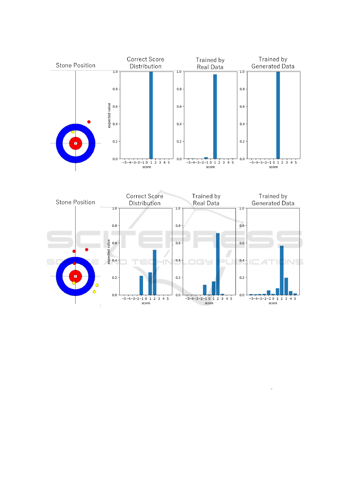
Figure 18: Stone position, correct score distribution and prediction results for each model in Situation 1. In this situation, the

score difference is 0, and the number of remaining ends is 0.

Figure 19: Stone position, correct score distribution and prediction results for each model in Situation 2. In this situation, the

score difference is -1, and the number of remaining ends is 0.

data and conduct training for cases other than the last

shot. Eventually, we would like to incorporate the

completed model into a curling AI and evaluate the

method through games on digital curling.

ACKNOWLEDGEMENTS

This work was supported by the “The Enhancement of

HPSC Infrastructure through Technology Innovation

Project” of Japan Sports Agency.

REFERENCES

Ataka, K., Noguchi, W., Iizuka, H., and Yamamoto, M.

(2020). Learning of evaluation function in digital curl-

ing considering the probability of scores at each end.

Proceedings of AAAI20 Workshop, Artiﬁcial Intelli-

gence in Team Sports, pages 1–6.

Curlit (2022). WWCC2022 resultsbook.

https://curlit.com/PDF/WWCC2022

ResultsBook.pdf.

Curlit (2024). Curling results. https://curlit.com/results.

Katoh, S., Iizuka, H., and Yamamoto, M. (2016). A

method of game tree search in digital curling includ-

ing uncertainty. Journal of Information Processing,

57(11):2354–2364.

icSPORTS 2024 - 12th International Conference on Sport Sciences Research and Technology Support

178

Figure 20: Stone position, correct score distribution and prediction results for each model in Situation 3. In this situation, the

score difference is 0, and the number of remaining ends is 0.

Myslik, J. (2020). Curling analytics.

https://www.jordanmyslik.com/portfolio/curling-

analytics/.

Uehara, K. and Ito, T. (2021). Improving the simula-

tor of digital curling to get closer to actual measure-

ment data. Technical Report 18, The University of

Electro-Communications,The University of Electro-

Communications.

Yamamoto, M., Katoh, S., and Iizuka, H. (2015). Digital

curling strategy based on game tree search. Proceed-

ings of 2015 IEEE Conference on Computational In-

telligence and Games, pages 474–480.

Yamamoto, M., Katoh, S., and Iizuka, H. (2018). Learning

of expected scores distribution for positions of digital

curling. Proceedings of Workshop on Curling Infor-

matics (WCI 2018), pages 8–9.

Creation of Training Data and Training for Prediction Model of Curling Scores Using Real Game Data

179