Reinforcement Learning for Autonomous Headland Turns

Lukas Pindl

, Riikka Soitinaho

, Patrick Behr

and Timo Oksanen

1,2

Chair of Agrimechatronics, Technical University of Munich (TUM), Germany

Munich Institute for Robotics and Machine Intelligence (MIRMI), Technical University of Munich (TUM), Germany

{lukas.pindl, riikka.soitinaho, timo.oksanen}@tum.de

Keywords:

Reinforcement Learning, Autonomous Vehicles, Agricultural Robotics, Headland Turning, Proximal Policy

Optimization.

Abstract:

This paper explores the use of reinforcement learning (RL) for the autonomous planning and execution of

headland turns, aiming to achieve real-time control without the need for preplanning. We introduce a method

based on proximal policy optimization (PPO), and incorporate expert knowledge through Dubins paths to

enhance the training process. Our approach models the vehicle kinematics and simulates the environment

in Matlab/Simulink. Results indicate that reinforcement learning (RL) can effectively handle the complexity

of headland turns, offering a promising solution for enhancing the efﬁciency and productivity of agricultural

operations. We show, that this approach can reach the turns goal point reliably in simulation with a positional

error of under 20 cm. We also test the policy on a real vehicle, showing that the approach can run in real

conditions, although with reduced accuracy. This study serves as a foundation for future research in more

complex scenarios and optimization goals.

1 INTRODUCTION

One main puzzle piece in the automatic coverage of

agricultural ﬁelds is the planning and execution of

headland turns. Headland turning involves the nav-

igation of machinery at the ends of crop rows dur-

ing ﬁeldwork activities such as plowing, planting, or

harvesting. The most common maneuvers are shown

in Figure 2. The headland, also known as the end

rows or turn rows, is a typically small area at the

edges of a ﬁeld where machinery turns to begin a new

pass. This practice, while seemingly straightforward,

plays a signiﬁcant role in the efﬁciency and productiv-

ity of farming. Efﬁcient headland turning minimizes

time loss, reduces soil compaction, and mitigates crop

damage, contributing to overall operational effective-

ness. Various factors, including equipment type, ﬁeld

geometry, and operator skill, inﬂuence the complex-

ity and execution of headland turns. Deep reinforce-

ment learning (DRL) is a potential option for this ap-

plication, that could allow for real time planning and

control of the vehicle. It could also enable inclusion

of multiple, sometimes competing, optimization ob-

jectives and should eventually be able to deal with

more complex vehicle models, due to it’s inherent

non-linearities. The goal for this paper is, to explore

the general viability of reinforcement learning (RL)

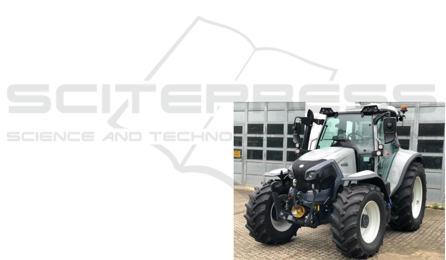
Figure 1: The AMX G-Trac is the chair’s own tractor. The

ﬁnal agent was able to do a headland turn with this vehicle.

for this task. We design the simulation to represent

our research tractor (see Figure 1), so that we can test

the ﬁnal agent on it.

To our knowledge, it is the ﬁrst example of an

RL based controller that can fully plan and execute

a headland turn without the need for any preplanning

in the ﬁeld. While the scope is still limited and some

simplifying assumptions are made, it is intended to

build a basis for future research with more complex

318

Pindl, L., Soitinaho, R., Behr, P. and Oksanen, T.

Reinforcement Learning for Autonomous Headland Turns.

DOI: 10.5220/0012944700003822

Paper published under CC license (CC BY-NC-ND 4.0)

In Proceedings of the 21st International Conference on Informatics in Control, Automation and Robotics (ICINCO 2024) - Volume 1, pages 318-325

ISBN: 978-989-758-717-7; ISSN: 2184-2809

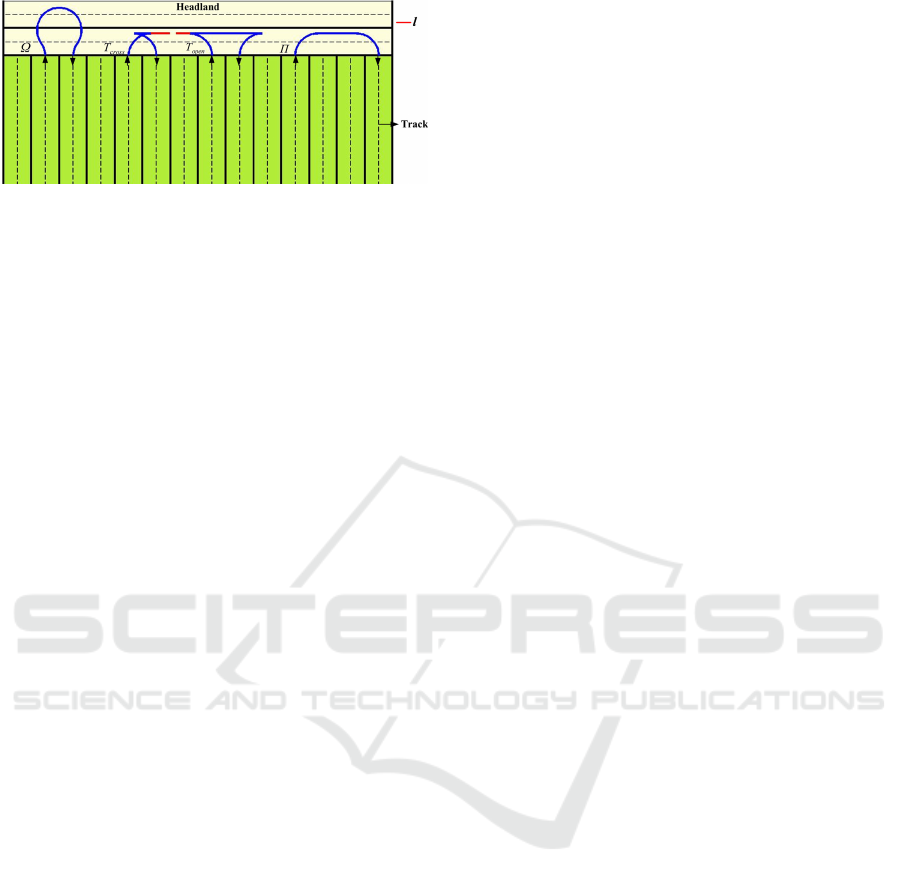
Figure 2: Illustration of the geometrical representation of a

ﬁeld with four common turn types: The forward turn (Ω-

Turn), the reverse cross turn (T

cross

or Fishtail-Turn), the

reverse open turn (T

open

) and the double round corner turn

(Π or U-Turn). (Zhou et al., 2015, Figure 5).

models and optimization goals.

2 BACKGROUND

2.1 Related Work

Headland turns can be planned with many different

approaches. The problem can be represented through

optimal control as in (Oksanen, 2007). Here, a numer-

ical solver is used to ﬁnd the necessary control inputs

and the resulting trajectory. This approach is revis-

ited by (Tu, 2013), where the solution is sped up with

some simpliﬁcations, as well as newer software and

hardware. (Sabelhaus et al., 2013) investigates the

use of continuous curvature paths for headland turns.

These use a similar approach as the well known Du-

bins turns (Dubins, 1957), but improve the real world

performance by accounting for limited steering rates.

(Cariou et al., 2009) and (Yin et al., 2020) plan a turn

using geometric approaches and use relatively simple

control laws to follow those trajectories. (Gao et al.,

2023) starts from scratch by also detecting the avail-

able headland area, mainly from camera images.

Much of the research regarding RL for non-

holonomic autonomous vehicles covers on-road driv-

ing. Off-road problems often have a very different

structure, making it necessary to ﬁnd separate solu-

tions. The agent designed by (Wiberg et al., 2022)

uses information about the goal position, several ve-

hicle states like joint angles and wheel slip as well

as a local height map to navigate a forestry vehicle

through rough terrain. (S

anchez et al., 2023) proposes

to learn steering actions end-to-end from lidar based

range measurements in uneven terrain with obstacles.

Curriculum learning is applied during training with a

generic actor-critic algorithm.

While parking often happens on paved areas, the

problem structure is still similar, with one goal pose

and a comparable vehicle model. (Lazzaroni et al.,

2024) simulates parking a car in the CARLA simu-

lator. The agent is trained in simulation to learn the

right throttle and steering controls from distance mea-

surements and goal information. Curriculum learning

is also applied. (Wu et al., 2023) let human volun-

teers park in the CARLA simulator to generate expert

knowledge, that is used to speed up training.

RL has not yet been extensively tested for either

planning or control of vehicles in an agricultural con-

text, but some examples exist. (Makino et al., 1999)

employ tabular RL to improve a globally generated

path for covering a ﬁeld. The vehicle model includes

an approximation of slip, that also depends on the ter-

rain.

(Olcay et al., 2023) train an agent to cover a ﬁeld

and successfully turn at the end of each lane. They

achieved this by predeﬁning a rough corridor, that the

vehicle should follow and then giving the DRL agent

its distance to the edge of this corridor in multiple di-

rections. A simple tractor-trailer kinematic model is

used for this purpose. Multiple learning algorithms

are applied and their results compared.

2.2 Headland Representation

Since the headland follows the edge of a ﬁeld, it can

have various shapes. In this paper, to simplify the

generation of different situations, we assume the ﬁeld

edge to be a straight line. While this is obviously not

true when looking at the entirety of a ﬁeld, this ap-

proximation is valid for most areas, as long as it is

only applied locally to a single turn. Such simpliﬁca-

tions are typical for headland turning automation (see

for example (Oksanen, 2007), (Tu, 2013), and (Yin

et al., 2020)). We only investigate left hand turns. For

the setup we use, to achieve a right hand turn, all in-

puts and outputs can simply be mirrored.

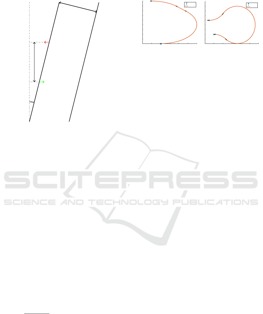
Figure 3 shows the geometrical representation that

we use in this paper. From any start pose p

start

the ﬁeld-headland edge x

h, field

(y) is easily deﬁned

through the headland angle α. The goal pose p

goal

can be calculated given the working width l

. Lastly,

the headland-outside x

h,out

(y) edge can be found by

shifting the ﬁeld-headland edge by a ﬁxed headland

width l

. Mathematically, these deﬁnitions can be for-

mulated as follows, if the start pose is assumed to be

start

= [0 0 0]

goal

= [l

sin(α) l

π]

(1a)

h, field

(y) = ysin(α) (1b)

h,out

(y) = l

cos(α) + y sin(α) (1c)

Reinforcement Learning for Autonomous Headland Turns

319

Field

Headland

h, f ield

Outside

Headland

h,out

start

goal

Figure 3: The general setup of the headland turn problem

for this paper. Arrows at start and goal point indicate the

vehicle orientation.

2.3 Proximal Policy Optimization

Proximal policy optimization (PPO) is an on-policy

actor-critic DRL method that was speciﬁcally de-

signed to allow the agent to be trained on samples

that were created with policies that were slightly dif-

ferent from the current one. PPO excels due to rel-

atively small computation times during the optimiza-

tion step, meaning that far more state-action pairs can

be included in training in the same amount of time.

PPO was introduced by (Schulman et al., 2017)

as a more computationally efﬁcient version of trust

region policy optimization (TRPO) (Schulman et al.,

2015). PPO clips the change of the policy to a maxi-

mum ratio ε. To achieve this, the probability of choos-

ing the action that was taken is stored for each sample

as π

old

) and the loss for the actor network is

then computed as

L (θ) = E

[min(r

(θ)A

,clip(k

(θ),1 − ε, 1 + ε)A

)]

(2a)

(θ) =

)

old

)

(2b)

with A

being the samples advantage. Note that the

ratio between the new and old policy k

(θ) is called

(θ) in the original paper. Since we use r for the re-

ward in this paper, we have changed the nomenclature

to avoid any confusion.

-2 -1 0 1 2 3 4

Start Position

Goal Position

Path

(a) U-Turn.

-2 0 2 4 6 8 10

-2

-1

Start Position

Goal Position

Path

(b) Ω-Turn.

Figure 4: Examples for a U-Turn and an Ω-Turn using Du-

bins connections.

2.4 Dubins Turns

A technique to ﬁnd optimal trajectories between two

points for any vehicle with a ﬁxed minimum turn ra-

dius is introduced by (Dubins, 1957). Some simpli-

fying assumptions are made, however. There is an

inﬁnite amount of free space in all directions, with no

obstacles. Another assumption that is not typically

true in real-life applications, is that the vehicle can

steer at any angle instantly. While the steering angle

is limited, leading to a minimum turn radius, the vehi-

cle needs to switch from a full left turn to a full right

turn in an instant to perfectly execute a Dubins turn.

Even with such limitations, these can however gener-

ate fairly good U-turns and Ω-turns as shown in Fig-

ure 4, that can be a starting off point for further learn-

ing. Dubins paths can always be split into 3 parts. The

ﬁrst is a curve, either left or right. Curves are always

at the minimum turn radius. The second part can ei-

ther be a straight segment, or a curve in the opposite

direction. The third segment is always a curve in the

same direction as the ﬁrst. This yields 6 different path

types. For each, the path can be geometrically con-

structed from the given circles and straight lines. The

shortest of the 6 paths is chosen. Because they are

relatively simple to generate, we use Dubins turns as

expert knowledge (see Section 4.2).

3 REINFORCEMENT LEARNING

ENVIRONMENT

3.1 Vehicle Model

The goal in this study is, to model the chairs agricul-

tural research tractor. It is a Lindner Lintrac 130, also

called the G-Trac, that can steer the rear wheels inde-

pendently. We therefore include the four wheel steer-

ing capability in the model for later use. However,

we ﬁx the rear wheel angle at δ

= 0 for all experi-

ments in this paper. The vehicle is modeled through

its kinematics only. The vehicle state is described by

ICINCO 2024 - 21st International Conference on Informatics in Control, Automation and Robotics

320

X = [x y ϕ δ

(3)

x and y are the vehicle’s coordinates, ϕ its heading,

,δ

describe the front and rear wheel angles and v

is the current velocity. The vehicle’s origin is set in

the center of the rear axle.

The kinematics are described by a simple differ-

ential equation, where l is the vehicle’s wheelbase:

dX =







vcos(ϕ)

vsin(ϕ)

(vsin(δ

− δ

)/(l cos(δ

)))







(4)

The control inputs for acceleration a and steering

rates ω

,ω

are limited by the given vehicle. For this

project, they are simply calculated from the desired

velocity and steering inputs, which were set by the

controller. To properly represent our G-Trac platform,

we used its wheelbase l = 2.42 m and maximum steer-

ing angle δ

f ,max

= 52

◦

in our simulation.

The ﬁrst three components of the vehicle state de-

scribe its pose p

= [x y ϕ]. This pose is based on the

position of the middle of the vehicle’s rear axle. It is

sometimes explicitly referred to as the rear pose. If

the position of the front axle is needed, it can be cal-

culated as

v, f

= p

+ [l cos(ϕ) l sin(ϕ) 0]

(5)

= [x

ϕ]

(6)

3.2 Observation + Action Space

The observation space contains all information that is

given to the agent. It can therefore have great im-

pact on it’s performance. Giving more values is usu-

ally better. However, information that doesn’t help the

agent make decisions, can simply slow down training.

It is unfortunately not always immediately obvious,

which values are useful and which are not.

Care should also be taken, that all observations

are realistically obtainable on the real-world vehicle.

Otherwise, the agent can not be transferred to the

ﬁeld.

The basic observation O for all experiments in this

paper is

O = [x

′

goal

′

goal

sin(ϕ

′

goal

) cos(ϕ

′

goal

) v d

α]

(7a)

′

goal

= [x

′

goal

′

goal

′

goal

], (7b)

= x

h, f ield

(y) − x

(7c)

′

goal

is the goal pose, but transformed into the ve-

hicle system. Sine and cosine are used here, to avoid

jumps in the angle at ±π. The horizontal distance to

the ﬁeld edge is given in d

. All values are also scaled

in the implementation, to keep values relatively small.

This helps with keeping gradients reasonable and sta-

bilizes learning.

To keep the setup simple, only the front steering

angle is controlled, meaning that the action space con-

sisted of only one variable, δ

3.3 Reward Function

The reward function is comprised of multiple compo-

nents. The full reward can be described as

f ull

= c

suc

− c

f ail

− c

time

(8a)

= max(|a

steer, f

| − 1.1δ

f ,max

,0) (8b)

suc

and r

f ail

are 1, when the vehicle is in a success

or failure condition, 0 otherwise (see Equation (9) and

10). a

steer, f

is the desired front wheel angle. Equa-

tion (8b) will lead to the steering reward r

being big,

if the desired angle is signiﬁcantly over the maximum

steering angle of the vehicle. This stops the agent

from getting stuck in a learned behavior, where ev-

ery action constantly exceeds the maximum allowed

value. The controller then caps the action to δ

f ,max

meaning that small, random changes still lead to the

same result. Exploration is then hindered, as all tested

actions are the same. This part of the reward is only

necessary, if the used algorithm does not limit the ac-

tion output, which is the case for the Matlab imple-

mentation of PPO.

A success was counted, when the vehicle pose was

close to the goal pose in both position and heading.

′2

goal

+ y

′2

goal

< ε

norm

(9a)

|ϕ

′

goal

| < ε

(9b)

The accuracy thresholds for the ﬁnal evaluation of

the policy are ε

norm

= 0.2;ε

, but different val-

ues are used during most of the training (see Sec-

tion 4.3). The failure condition is reached, if the front

axle passes the headland-outside edge, or if the rear

axle passes from the headland into the ﬁeld by more

than 1 m:

< 0 (10a)

x < x

h, f ield

(y) − 1 (10b)

Typical values for the scaling factors in training

are c

suc

= 1, c

f ail

= 1, c

= 0.002, c

time

= 0.001.

Reinforcement Learning for Autonomous Headland Turns

321

4 IMPLEMENTATION

4.1 Matlab/Simulink Setup

The vehicle model described in Section 3.1 is imple-

mented in Simulink. The differential equation Equa-

tion (4) is solved in discrete time steps of ∆t = 100ms

through a simple integrator. The control block re-

ceives the current state from this simulation and sends

the next steering angle as a control input. Inside the

control block, the vehicle state is used in conjunction

with the current scenario parameters to compute the

agent’s observations. The Simulink RL Agent block

is used to easily learn and execute the policy. A vi-

sualization is also provided, which can be turned off

during training.

The training setup is done in Matlab scripts. This

includes the reset function for the environment. At

the start of each episode, the agent starts at the origin

and the headland angle is chosen at random between

±30

◦

4.2 Inclusion of Expert Knowledge

Using purely random actions, the agent is extremely

unlikely to reach the goal without exiting the head-

land area. With so little positive reward, the agent

will probably not learn a successful policy. To avoid

this problem, agents can be pretrained from expert

knowledge, that is at least good enough to get close

to the goal, some of the time. For this purpose, Du-

bins turns, as introduced in Section 2.4, are used in

this paper. At the start of each episode, the inbuilt

Matlab function for generating Dubins turns is em-

ployed. This function outputs the distances, for which

the vehicle has to drive at a full left/right turn. This

information is used to directly control the vehicle in

simulation, by continuously integrating the distance

traveled, and changing the steering angle accordingly.

Since only tight, left-hand turns were tested for

this paper, all turns are of the type right-left-right.

Since the vehicle model uses limited steering rates,

strictly following these turns leads to a signiﬁcant

mismatch. By simply adjusting the distance for each

of the 3 stages of the turn by a constant length, a much

better result can be achieved. For the speciﬁc setup in

this paper, the three stages are changed by -0.5m, -

0.8m and +0.1m respectively. While this is by far not

sufﬁcient for reaching the goal very accurately and

consistently (see Table 2), it is good enough to give

some positive examples to the agent, allowing it to

learn from there.

The decision whether the agent will follow its cur-

rent RL policy or this expert knowledge, is made ran-

Table 1: Hyperparameters used for the most successful

training with PPO. Bold Parameters were varied in the ran-

dom search.

Parameter Value

Learning Rate Actor (Part 1) 5.448 × 10

−5

Learning Rate Actor (Part 2) 9.712 × 10

−6

Learning Rate Critic (Part 1) 3.202 × 10

−5

Learning Rate Critic (Part 2) 1.030 × 10

−5

Action Log Prob (Part 2) −2.677

Experience Horizon 4096

Minibatch Size 256

Clip Factor 0.1

Discount Factor 0.995

EntropyLossWeight 0.001

domly at the beginning of each episode. The chance

of using expert knowledge starts at almost 100%, and

is lowered linearly with the number of episodes all the

way to 0% shortly before the end of training.

4.3 Training and Hyperparameters

The Matlab RL-Pipeline makes it hard to dynamically

change certain hyperparameters during training. To

allow for fast learning in the beginning, but accurate

adjustments in the end, the training is split into two

parts, where the learning rates are lowered for the sec-

ond one. In the secondary training, the log probabil-

ity of the action’s normal distribution is also set to a

ﬁxed value. The ﬁrst training is for 17000 episodes,

the second for 5000. The second training is started

from the saved model that achieved the best success

rate at 20 cm accuracy during the ﬁrst training. Af-

ter manual tuning to ﬁnd a good baseline, a random

search over the most impactful hyperparameters is

performed. The agent with the best performance was

trained using the values listed in Table 1. Parameters

that are not mentioned use the default values in the

Matlab PPO implementation.

Even with the initial use of pregenerated Dubins

turns the agent would fail most attempts at the start

of the training. A lack of positive reinforcement can

make it harder for the algorithm to learn the desired

behavior. To increase the likelihood of success, the

values for ε

norm

,ε

as introduced in Section 3.3 are

initially set to fairly high values (typically 1.5 m and

). As the training progresses the difﬁculty is in-

creased by lowering these thresholds. In the best

case, this would be done dynamically, whenever the

agent reaches sufﬁcient success rates on the current

difﬁculty. Due to limitations with the learning setup

in Matlab, this was not easily possible. Instead, the

thresholds where lowered linearly over the course of

the training and reached their minimum shortly before

the episode limit of the training was reached. Chang-

ing the difﬁculty throughout the process brings some

ICINCO 2024 - 21st International Conference on Informatics in Control, Automation and Robotics

322

problems with it. The learning rate must be very well

tailored to the rate at which the thresholds are ad-

justed. Otherwise the agent either overﬁts to the cur-

rent difﬁculty, or the agent can not keep up with the

increase in difﬁculty. In the end, a good balance was

found that allowed the agent to slowly adjust to the

new thresholds.

4.4 Real World Vehicle Integration

For testing the ﬁnal policy in the real world, we use

the G-Trac that the chair has modiﬁed with multiple

sensors and controllers. The position of the vehicle is

gained from an RTK-GNSS receiver. From the posi-

tion of the antenna as well as current pitch and roll an-

gles from an IMU sensor, the position of the rear axle

near the ground can be calculated. An interface on the

G-Trac allows controlling the speed and steering an-

gles. The data is sent via CAN-Bus to the G-Trac at

a rate of 10 Hz, which then executes the commanded

actions. The G-Trac is shown in Figure 1. The pol-

icy was tested on a sloped grass ﬁeld as well as a ﬂat,

paved yard.

5 RESULTS

5.1 Training Progression

The results shown in this section are for the most suc-

cessful agent found during the hyperparameter search,

as discussed in Section 4.3. The agent learned to com-

plete a 3 m turn (l

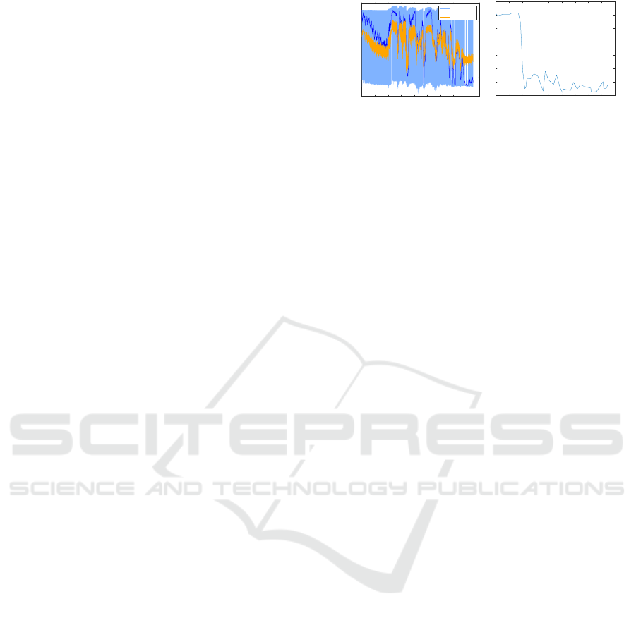
= 3). Figure 5a indicates, how the

cumulative reward per episode developed. The dark

blue line shows the average reward over the previ-

ous 100 episodes. The yellow line tracks the critics

prediction in the ﬁrst step of the episode, which in-

cludes the discount factor γ. The early decline of the

reward is expected, since the difﬁculty is increasing.

The ratio of precomputed Dubins turns to RL based

episodes is decreasing at the same time. At around

5000 episodes the steep improvement indicates that

the agent has managed to learn how to complete turns

for most of the tested headland angles at this point.

The frequent drops are most likely due to overﬁt-

ting to the current difﬁculty, meaning that the learning

rate may have been just slightly too high. The agent

was mostly able to recover however. The ﬁnal accu-

racy required to be considered successful was set at

10 cm. Since actions are drawn semi-randomly dur-

ing training, this threshold could rarely be reached,

leading to the ﬁnal episodes getting fairly low re-

wards. During training the agent is saved regularly,

when performance is especially good. This consists

0 2000 4000 6000 8000 10000 12000 14000 16000 18000

Episodes

-1.5

-1

-0.5

0.5

Reward

Episode Reward

Moving Average

First Step Critic

(a) Reward.

0 2000 4000 6000 8000 10000 12000 14000 16000 18000

Episodes

0.5

1.5

2.5

3.5

Root Mean Squared Error

(b) RMSE.

Figure 5: Indicators for training progression with the basic

setup.

of checking if a new global or local maximum was

reached in the average reward. To avoid saving too

many models, which would have signiﬁcant storage

and time costs, some hysteresis is added. Then the

performance of each saved model is tested: The agent

is set to always choose the mean of the action dis-

tribution. With this deterministic agent 100 random

episodes are completed. For each episode the error

is computed as the smallest distance that the vehicle

ever had to the target. In our test we let the agent drive

past the goal to ﬁnd this minimal distance, meaning

that the last recorded position was further away from

the goal than the best one. In a real application, it

would more likely be stopped as soon as the distance

starts increasing again. The way we measure the root

mean squared error (RMSE) reﬂects the second ap-

proach. Figure 5b shows how the resulting RMSE

progressed over training. While it clearly had a ma-

jor improvement around 4000 episodes, the value still

varies strongly afterwards, indicating that the training

was not especially stable.

5.2 Generated Trajectories

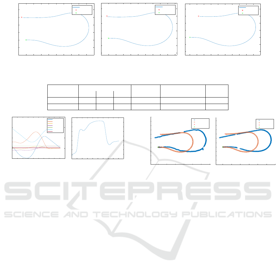
As expected, the ﬁnal results are similar to the Du-

bin’s turns, which we use as expert knowledge. To

successfully ﬁnish a 3 m turn, the vehicle needs to

steer right ﬁrst, then do the left turn, and ﬁnally steer

back to straighten out the tractor. This can be seen in

the trajectories in Figure 6, as well as in the generated

actions in Figure 7b. Since we are using the deter-

ministic policy for evaluation, we can also see, that

the actions are fairly smooth. There is some minor

overcorrection in the desired steering angle at around

steps 30-40. It is likely that a trajectory without this

correction would be faster, but the agent simply is not

able to learn this. It is a good example of a situation

where the blackbox type approach of artiﬁcial neu-

ral networks (ANNs) makes it very hard to ﬁnd the

exact reasoning for the selected action. All generated

turns reached within 20 cm of the target point. Table 2

shows the metrics we used to evaluate how well the ﬁ-

nal agent did on different difﬁculties. Comparing the

Reinforcement Learning for Autonomous Headland Turns

323

-1 0 1 2 3 4 5 6 7 8 9

x (m)

-2

-1

y (m)

Headland Angle: -11.3337°

vehicle path

target

start

-1 0 1 2 3 4 5 6 7 8 9

x (m)

-2

-1

y (m)

Headland Angle: -4.1876°

vehicle path

target

start

0 1 2 3 4 5 6 7 8 9 10

x (m)

-2

-1

y (m)

Headland Angle: 24.2928°

vehicle path

target

start

Figure 6: Paths generated for multiple headland angles with the basic setup.

Table 2: Success Metrics, tested on random headland angles. TTS is time to success. Results over 1000 episodes.

Strategy Success Rate (%) RMSE (m) Heading RMSE (°) TTS (s)

0.1m 0.2m 0.5m 0.2m

Dubins turn 27.0 32.8 63.7 0.873 3.71 22.16

PPO agent 32.4 100 100 0.133 1.83 20.35

0 20 40 60 80 100 120 140 160 180 200

Step

-5

State Value

x error (m)

y error (m)

phi error (sin)

phi error (cos)

velocity (m/s)

dist to edge (m)

headland angle

(a) Observations.

0 20 40 60 80 100 120 140 160 180 200

Step

-0.8

-0.6

-0.4

-0.2

0.2

0.4

0.6

0.8

desired steering angle

(b) Generated Action.

Figure 7: Inputs and outputs to the RL agent with the basic

setup.

metrics to the untrained Dubins turns, that are used

as expert knowledge to initiate the training, it is clear

that the trained agent performs signiﬁcantly better in

all categories.

During training, the heading is an important part

of deciding whether or not an episode was successful

or not (see Equation (9)). This means, that the agents

learns to line up with the intended ﬁnal heading. For

the success rates shown in Table 2, this angle is not

checked. This is mainly to keep the difﬁculty cate-

gories simpler, since it is hard to decide which head-

ing threshold to combine with which distance thresh-

old. The heading error shown in the tables is the angle

that was reached for the time step that was closest to

the goal in distance. It is possible, that there is a time

step in the turn, where the sum of positional and an-

gular error is smaller, but this point would depend on

the weight that we would apply to either error. We

instead opt to just use the point with the lowest posi-

tional error. The time to success was also measured to

this time step. Since a constant velocity is used, this

value directly corresponds to the distance traveled.

5.3 Real World Vehicle

A total of 7 turns with the RL agent were performed

on the G-Trac on different surfaces. One of the turns

0 2 4 6 8 10 12

x (m)

-4

-3

-2

-1

y (m)

gtrac path

simulated path

target

start

(a) Field.

0 2 4 6 8 10 12

x (m)

-4

-3

-2

-1

y (m)

gtrac path

simulated path

target

start

(b) Yard.

Figure 8: Paths generated in the real world using the G-

Trac.

had to be excluded from the results. It automatically

stopped in the middle of the turn without any of the

normal failure conditions being met. This was most

likely due to a conﬁguration error, that had nothing to

do with the agent itself.

Figure 8 shows 2 of the recorded turns. Since

all turns have very similar performance, the ones in

the ﬁgure are simply chosen for how complete the

recorded position data is. The ones that are presented

have the least amount of GNSS gaps, making them

more useful for visual inspection. In the performance

metrics, no major differences between the different

surfaces can be seen. All of them are therefore com-

bined in the results: Only one turn reaches the goal

within 50 cm, but all reach within 60 cm. The RMSE

is 0.532 m. The average time to reach the closest point

to the goal pose is 42.5 s. The ﬁnal heading error is

relatively high with an average error of 12.6

◦

Figure 8 also shows the agent’s path in the simu-

lation for the same headland angle. It is obvious that

the tractor behaves differently in real life, leading to

a longer turn. This results in observations that were

never seen during training. The agent still manages

to turn with these unexpected observations, but fails

to correct in the ﬁnal stages. The fact that this small

difference stops the agent from ﬁnishing correctly in-

ICINCO 2024 - 21st International Conference on Informatics in Control, Automation and Robotics

324

dicates that it has overﬁtted to the simulated environ-

ment.

6 DISCUSSION AND

CONCLUSION

The results show that an RL based agent is capable of

planning a headland turn and controlling the vehicle

to follow it. The ﬁnal policy can easily be executed

in under 100ms, meaning that the approach is viable

for running in real time. However, the stability of the

training is still somewhat lacking. While we are able

to ﬁnd a great policy even with the instability, improv-

ing on this would be desirable to speed up training and

allow for more difﬁcult problems.

Since this paper is intended as a proof-of-concept,

no in-depth comparison to other headland turning al-

gorithms is made. This should be an important com-

ponent for future research into the area.

It is also clear that this implementation does not

use many of the theoretical advantages of RL. Re-

search that focuses on using more complex vehicle

models and optimization goals could greatly beneﬁt

from those strengths.

For the real world application, more techniques to

improve the sim-to-real transfer could be applied. The

results could likely be improved signiﬁcantly, if the

policy was forced to achieve better generalization.

ACKNOWLEDGMENTS

We would like to thank Michael Maier and Ruben

Hefele for their help with implementing and testing

the policy on the real tractor. We are also very great-

ful for Henri Hornburg’s input on possible algorithms

for the expert knowledge generation.

REFERENCES

Cariou, C., Lenain, R., Thuilot, B., and Martinet, P.

(10.10.2009 - 15.10.2009). Motion planner and

lateral-longitudinal controllers for autonomous ma-

neuvers of a farm vehicle in headland. In 2009

IEEE/RSJ International Conference on Intelligent

Robots and Systems, pages 5782–5787. IEEE.

Dubins, L. E. (1957). On Curves of Minimal Length with a

Constraint on Average Curvature, and with Prescribed

Initial and Terminal Positions and Tangents. American

Journal of Mathematics, 79(3):497.

Gao, G., Guo, H., Zhang, J., Zhang, Z., Wu, T., Lu, H.,

Qiu, Z., Chen, H., and Lingxuan, Z. (2023). An ef-

ﬁcient headland-turning navigation system for a saf-

ﬂower picking robot. Journal of Agricultural Engi-

neering, 54(3).

Lazzaroni, L., Pighetti, A., Bellotti, F., Capello, A., Cossu,

M., and Berta, R. (2024). Automated Parking in

CARLA: A Deep Reinforcement Learning-Based Ap-

proach. In Bellotti, F., Grammatikakis, M. D., Man-

sour, A., Ruo Roch, M., Seepold, R., Solanas, A., and

Berta, R., editors, Applications in Electronics Pervad-

ing Industry, Environment and Society, volume 1110

of Lecture Notes in Electrical Engineering, pages

352–357. Springer Nature Switzerland.

Makino, T., Yokoi, H., and Kakazu, Y. (28-30 July 1999).

Development of a motion planning system for an agri-

cultural mobile robot. In SICE ’99. Proceedings of

the 38th SICE Annual Conference. International Ses-

sion Papers (IEEE Cat. No.99TH8456), pages 959–

962. Soc. Instrum. & Control Eng.

Oksanen, T. (2007). Path planning algorithms for agricul-

tural ﬁeld machines, volume no. 31 0031 of Helsinki

University of Technology Automation Technology

Laboratory Series A Research reports. Helsinki Uni-

versity of Technology, Espoo.

Olcay, E., Rui, X., and Wang, R. (26.08.2023 - 30.08.2023).

Headland Turn Automation Concept for Tractor-

Trailer System with Deep Reinforcement Learning.

In 2023 IEEE 19th International Conference on Au-

tomation Science and Engineering (CASE), pages 1–

7. IEEE.

Sabelhaus, D., R

oben, F., Meyer zu Helligen, L. P., and

Schulze Lammers, P. (2013). Using continuous-

curvature paths to generate feasible headland turn ma-

noeuvres. Biosystems Engineering, 116(4):399–409.

anchez, M., Morales, J., and Mart

ınez, J. L. (2023). Re-

inforcement and Curriculum Learning for Off-Road

Navigation of an UGV with a 3D LiDAR. Sensors

(Basel, Switzerland), 23(6).

Schulman, J., Levine, S., Moritz, P., Jordan, M. I., and

Abbeel, P. (2015). Trust Region Policy Optimization.

Schulman, J., Wolski, F., Dhariwal, P., Radford, A., and

Klimov, O. (2017). Proximal Policy Optimization Al-

gorithms.

Tu, X. (2013). Robust navigation control and headland

turning optimization of agricultural vehicles. PhD

thesis, Iowa State University.

Wiberg, V., Wallin, E., Nordfjell, T., and Servin, M. (2022).

Control of Rough Terrain Vehicles Using Deep Rein-

forcement Learning. IEEE Robotics and Automation

Letters, 7(1):390–397.

Wu, Y., Wang, L., Lu, X., Wu, Y., and Zhang, H.

(27.10.2023 - 29.10.2023). Reinforcement Learning-

based Autonomous Parking with Expert Demonstra-

tions. In 2023 7th CAA International Conference on

Vehicular Control and Intelligence (CVCI), pages 1–

6. IEEE.

Yin, X., Wang, Y., Chen, Y., Jin, C., and Du, J. (2020).

Development of autonomous navigation controller for

agricultural vehicles. International Journal of Agri-

cultural and Biological Engineering, 13(4):70–76.

Zhou, K., Jensen, A. L., Bochtis, D. D., and Sørensen, C. G.

(2015). Quantifying the beneﬁts of alternative ﬁeld-

work patterns in a potato cultivation system. Comput-

ers and Electronics in Agriculture, 119:228–240.

Reinforcement Learning for Autonomous Headland Turns

325