Using Shapley Additive Explanations to Explain a Deep Reinforcement

Learning Agent Controlling a Turtlebot3 for Autonomous Navigation

Sindre Benjamin Remman

and Anastasios M. Lekkas

Department of Engineering Cybernetics, Norwegian University of Science and Technology (NTNU), Trondheim, Norway

{sindre.b.remman, anastasios.lekkas}@ntnu.no

Keywords:

Explainable AI, Deep Reinforcement Learning, Shapley Additive Explanations, LiDAR Data.

Abstract:

We employ Shapley Additive Explanations (SHAP) to interpret a DRL agent’s decisions, trained using the

Soft-Actor Critic algorithm for controlling a TurtleBot3 via LiDAR in a simulated environment. To leverage

spatial correlations between laser data points, we use a neural network with a convolutional ﬁrst layer to

extract features, followed by feedforward layers to choose actions based on these extracted features. We use

the Gazebo simulator and Robotic Operating System (ROS) to simulate and control the TurtleBot3, and we

implement visualization of the calculated SHAP values using rviz, coloring the LiDAR states based on their

SHAP values. Our contributions are as follows: (1) To our knowledge, this is the ﬁrst research paper using

the SHAP method to explain the decision-making of a DRL agent controlling a mobile robot using LiDAR

data states. (2) We introduce a visualization approach by clustering LiDAR data points using Density-based

spatial clustering of applications with noise (DBSCAN) and visualizing the average SHAP values for each

cluster to improve interpretability. Our results show that although the agent often makes decisions based on

human-interpretable information, such as an obstacle on the left necessitating a right turn and vice versa, the

agent has also learned to use information that is not human-interpretable. We hypothesize and discuss if this

indicates the policy is overﬁtted to the map used for gathering data.

1 INTRODUCTION

Recent developments in deep reinforcement learning

(DRL) have demonstrated remarkable performance

across diverse domains, ranging from video games

(Badia et al., 2020) to robotic control (Brunke et al.,

2022). However, understanding the decision-making

of DRL agents remains a signiﬁcant challenge due to

their neural network-based policies. This lack of in-

terpretability impedes the diagnosis and improvement

of agent performance in control tasks, particularly in

safety-critical applications.

To tackle the interpretability challenges of DRL

agents, researchers in Explainable Artiﬁcial Intelli-

gence (XAI) have developed various methods to en-

hance the explainability of DRL models. Such meth-

ods can offer insights into the DRL models’ decision-

making processes and lead to improved performance,

better debugging, and increased trust in these systems.

One widely used method in the XAI community is

Shapley Additive Explanations (SHAP), which is a

https://orcid.org/0009-0005-7593-5913

https://orcid.org/0000-0001-6885-6372

feature attribution method. This type of method aims

to determine the contribution of each input feature to

the output made by an machine learning (ML) model.

SHAP is especially popular due to its strong theo-

retical foundation in cooperative game theory, which

guarantees fair and consistent distribution of feature

importance. This foundation allows SHAP to satisfy

certain properties, such as

• Local Accuracy. The explanation model’s pre-

diction should match the original model’s predic-

tion for any given instance.

• Missingness. Features not present in the model

should have no attributed importance.

• Consistency. If a model changes so that it relies

more on a feature, the SHAP value for that feature

should not decrease.

These properties set SHAP apart from other feature

attribution methods, making it a robust and reliable

tool for interpretability.

In this paper, we employ SHAP to explain a DRL

agent trained with the Soft Actor-Critic (SAC) algo-

rithm to control a TurtleBot3 for autonomous navi-

gation. The TurtleBot3 operates in a simulated in-

334

Remman, S. and Lekkas, A.

Using Shapley Additive Explanations to Explain a Deep Reinforcement Learning Agent Controlling a Turtlebot3 for Autonomous Navigation.

DOI: 10.5220/0012950200003822

Paper published under CC license (CC BY-NC-ND 4.0)

In Proceedings of the 21st International Conference on Informatics in Control, Automation and Robotics (ICINCO 2024) - Volume 1, pages 334-340

ISBN: 978-989-758-717-7; ISSN: 2184-2809

door environment, using a 360° LiDAR sensor to per-

ceive its surroundings and navigate through an obsta-

cle course. While this type of navigation can be ef-

fectively solved with traditional methods, it serves as

a valuable test environment for our purposes. Dur-

ing future work, we can easily apply the policy to a

real Turtlebot3 because of its safe operation, and later,

we can include complications where DRL offers ad-

vantages, such as dynamic obstacles and humans in

the environment. We visualize the SHAP values of

each LiDAR point state in rviz by coloring the Li-

DAR readings by their SHAP value. Speciﬁcally, the

contributions of this paper are:

• To our knowledge, this is the ﬁrst research paper

using SHAP to explain the decision-making of a

DRL agent controlling a mobile robot using Li-

DAR data states.

• We show how feature attributions for LiDAR data

features, such as ones generated by SHAP, can be

visualized in rviz by coloring the LiDAR points

by their SHAP value. To improve the visualiza-

tion, we cluster the laser data using DBSCAN and

visualize each cluster’s average SHAP values.

1.1 Related Work

Work has already been done on using the TurtleBot3

to navigate environments using DRL. The authors in

(Cimurs et al., 2022) use DRL for local navigation

to move between waypoints toward a global goal in

an unknown environment. The waypoints are gen-

erated through a global navigation scheme based on

a map that is continuously updated using simultane-

ous localization and mapping (SLAM). This approach

is similar to ours, although we do not implement a

higher-level global navigation scheme. Instead, we

assign a randomly selected goal waypoint for each

episode. The way we use SHAP to explain the DRL

policy could easily be adapted to the approach in

(Cimurs et al., 2022).

Although there has not been much work done on

using feature attributions to explain DRL agents with

LiDAR data states, there has been signiﬁcant work

on feature attribution methods for explaining DRL

agents with other types of state spaces. In (Gjærum

et al., 2023), the authors use model trees as surro-

gate models to create feature attributions explaining

a DRL agent. The authors in (Remman et al., 2022)

compare two variants of SHAP, Kernel SHAP and

Causal SHAP on a robotic DRL task involving ma-

nipulating a lever using a robotic manipulator. In

(Bellotti et al., 2023), the authors propose a frame-

work to interpret the behavior of DRL agents in a

highway simulation environment using three types of

analysis: episode timeline, frame-by-frame, and ag-

gregated statistical analysis. The authors used SHAP

and attention mechanisms to understand the agents’

decision-making process.

2 PRELIMINARIES

2.1 Shapley Additive Explanations

Shapley Additive Explanations (SHAP), which was

introduced in (Lundberg and Lee, 2017), is a feature-

attribution method, which means that it explains how

much each input to an ML model contributes to the

output of the model. SHAP has its roots in coopera-

tive game theory and is based on the Shapley decom-

position, introduced by Lloyd Shapley in 1953 (Shap-

ley, 1952). This decomposition fairly assigns parts of

the outcome of a game to the game’s players based

on their contribution to the game’s outcome. In the

context of SHAP, these ”players” are the input fea-

tures, and the game’s outcome is the output of the ML

model. The Shapley value ensures a fair distribution

of contributions by representing the average marginal

contribution of each feature across all possible coali-

tions of features (Molnar, 2022):

∑

S⊆N\{i}

|S|!(|N|−|S|−1)!

|N|!

[ f (S ∪{i}) − f (S)]

(1)

Here, φ

represents the Shapley value for feature i,

N is the set of all features, S is a subset of N excluding

i, and f is the model’s prediction function. This for-

mula considers all possible subsets S, making SHAP

values computationally intensive to calculate exactly.

In addition, it is generally impossible to evaluate neu-

ral network models with missing features.

Several approximation methods have been devel-

oped to make SHAP values feasible for real-world

applications. Among them, Deep SHAP and Kernel

SHAP are widely used:

• Deep SHAP is tailored for deep learning mod-

els and leverages neural network structure to ef-

ﬁciently approximate SHAP values.

• Kernel SHAP is a model-agnostic method that

approximates SHAP values using a weighted lin-

ear regression model, suitable for any machine

learning model.

Deep SHAP generates explanations much faster than

Kernel SHAP by leveraging neural network-speciﬁc

features, such as backpropagation and GPU accelera-

tion. Our experiments, therefore, used Deep SHAP to

generate the explanations.

Using Shapley Additive Explanations to Explain a Deep Reinforcement Learning Agent Controlling a Turtlebot3 for Autonomous

Navigation

335

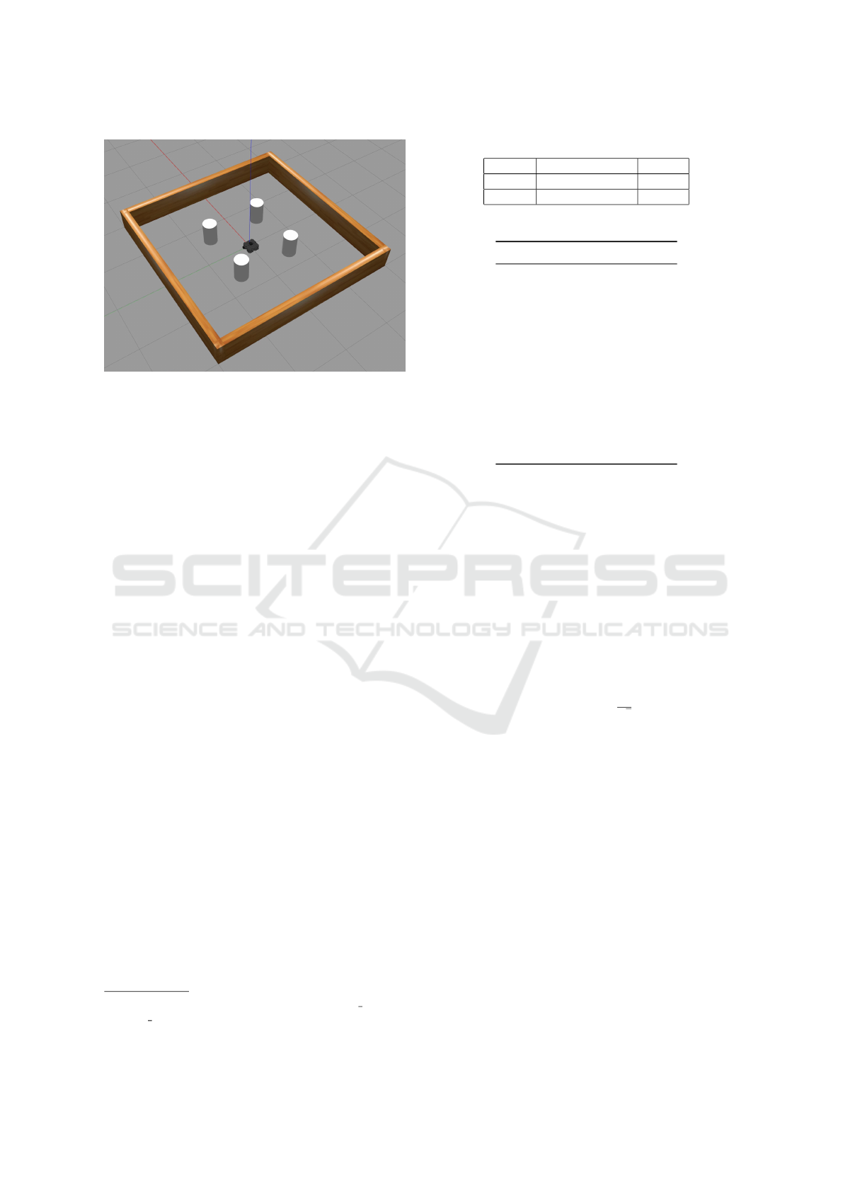
Figure 1: The second environment from the TurtleBot3 ma-

chine learning package.

3 METHODOLOGY

3.1 Experimental Setup

We train the SAC policy in the Gazebo simulator

(Koenig and Howard, 2004) and control the simu-

lated robot using ROS commands (Quigley et al.,

2009). We base the implementation of our reinforce-

ment learning environment on the TurtleBot3 ma-

chine learning package

. This implementation uses a

discrete action space and some redundant information

in the state space, such as the angle and distance to the

nearest obstacle. This information is already a part of

the LiDAR reading states. The robot also always has a

0.15 m/s linear velocity, and only the angular velocity

is controlled using the actions.

We adapt the implementation to better suit our

purposes by changing both the state space, action

space, and reward function. These changes are de-

tailed below, in Section 3.2. The map on which we

base our experiments is the second environment of

the TurtleBot3 machine learning package, which is

shown in the Gazebo simulator in Figure 1. This

environment has four columns spaced symmetrically

around the center and four walls encasing the envi-

ronment. The TurtleBot3 starts every episode in the

middle of the environment, as in Figure 1.

3.2 Problem Formulation and Solution

The reinforcement learning (RL) problem we address

is navigating the TurtleBot3 from the center of the en-

vironment shown in Figure 1 to a randomly selected

https://github.com/ROBOTIS-GIT/turtlebot3

machine learning.git

Table 1: Deﬁnition of actions and their respective ranges.

Action Description Range

Linear velocity [−1, 1]

Angular velocity [−1, 1]

Table 2: The hyperparameters used for SAC.

Hyperparameter Description

Learning Rate 0.0003

Gamma 0.99

Batch Size 256

Replay Buffer Size 1000000

Entropy Coefﬁcient auto

Update Interval 1

Gradient Steps 1

Training Time Steps 1000000

Optimizer Adam

Conv1d Filters 1

Conv1d Kernel Size 20

Conv1d Stride 5

Conv1d Padding 5

position within the outer walls. The state space S con-

sists of 180 readings from the TurtleBot3’s 360° Li-

DAR, as well as two states with the distance to the

goal and the angle from the heading direction to the

goal position, represented as a 182-dimensional vec-

tor of continuous values s ∈ S .

The action space A is continuous, with each ac-

tion a ∈ A consisting of two entries, as deﬁned in Ta-

ble 1. In this case, a negative angular velocity makes

the TurtleBot3 turn towards its right. We deﬁne our

reward function as follows:

R(s, a) =











200 if goal reached

−200 if collision

−(distance to goal)

√

otherwise

which we found to work well through trial and error.

To solve this environment, we train our policy us-

ing the Stable-Baselines3 implementation of the SAC

algorithm (Rafﬁn et al., 2021) (Haarnoja et al., 2018).

The hyperparameters used for training the policy are

shown in Table 2.

3.3 SHAP Explanation and

Visualization

To better understand how the agent solves the RL en-

vironment, we employ SHAP. We use the SHAP ex-

plainer to compute SHAP values from the inputs to

the policy (LiDAR data and the distance and heading

to the goal) to the mean action chosen by the policy.

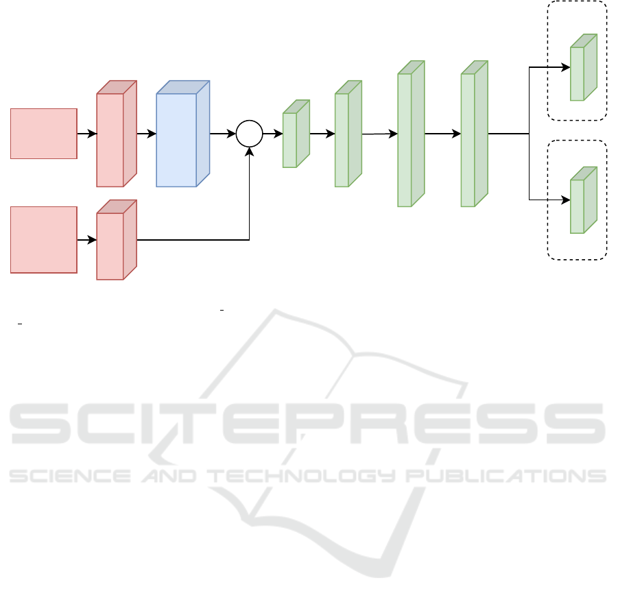
This action is obtained by applying the Tanh activa-

tion function after the µ layer, as shown in Figure 2.

We are primarily interested in understanding how the

ICINCO 2024 - 21st International Conference on Informatics in Control, Automation and Robotics

336

Input |180

FC|256

FC|128

Conv1d

LiDAR

Data

Goal

distance

and angle

Input |2

FC|37

FC|256

FC|2

log_std

FC|2

Figure 2: This ﬁgure shows the SAC actor network used. After the Conv1d layer and all fully connected (FC) layers except

the two last FC layers marked by µ and log std, there are rectiﬁed linear unit (ReLU) activation functions. After the µ and

log

std layers, there are hyperbolic tangent (Tanh) activation functions.

LiDAR states contribute to the actions chosen by the

policy. To visualize this, we overlap the SHAP val-

ues with the LiDAR readings, coloring them blue for

negative SHAP values and red for positive ones. The

more deeply they are colored, the greater the mag-

nitude of the SHAP value. Negative SHAP values

decrease the model output, while positive values in-

crease it. In our case, negative SHAP values con-

tribute to more negative actions: for Action 1, this

means a more negative linear velocity, and for Action

2, a more negative angular velocity. We display this

visualization in rviz by publishing the colored LiDAR

readings on a ROS topic as Marker messages. An ex-

ample of this visualization can be seen in Figure 3.

To generate new SHAP values in as close to real-

time as possible, we use Deep SHAP from the SHAP

Python library. In contrast to the widely used Ker-

nel SHAP, Deep SHAP can generate much faster. In

our experiments, we could generate SHAP explana-

tions using Deep SHAP at an average rate of 14.533

Hz, while Kernel SHAP generated explanations at an

average rate of 0.444 Hz.

To make the visualization of the SHAP values

more suitable for real-time examination, we used

density-based clustering to group the LiDAR data

points and subsequently visualize the average SHAP

value for each of these clusters. This approach was

chosen to address the noise present in the SHAP val-

ues, which made them challenging to interpret. For

the clustering, we used the DBSCAN method to clus-

ter together dense regions of LiDAR points (Ester

et al., 1996).

4 RESULTS AND DISCUSSION

In the ﬁrst part of this section, we discuss how apply-

ing SHAP to our RL problem yields results that align

with human intuition. For example, LiDAR readings

corresponding to nearby obstacles contribute to ac-

tions that move the TurtleBot3 away from those ob-

stacles. Next, we discuss how the policy has learned

to look at parts of the LiDAR readings that are not

necessarily human-understandable. Finally, because

of the at times noisy SHAP values, we implement a

density-based clustering scheme using DBSCAN to

simplify the visualization.

4.1 Human-Interpretable SHAP Values

When the TurtleBot3 has to move close to or towards

an obstacle to reach its goal, the LiDAR readings cor-

responding to that obstacle are often given SHAP val-

ues, which indicate that these readings tell the pol-

icy to keep away from them. From Figure 3, we can

see this is the case when the goal is located between

and beyond two of the columns in the environment.

This plot shows the SHAP values for action 2, which,

as discussed in Section 3.2, is the action that sends

an angular velocity command to the TurtleBot3. The

left-forward column is mainly colored blue, which

indicates that this column contributes to decreasing

action 2, which, in return, makes the angular veloc-

ity command more negative. Compare this to the

right-forward column, which is primarily colored red.

These SHAP values indicate that the policy uses the

Using Shapley Additive Explanations to Explain a Deep Reinforcement Learning Agent Controlling a Turtlebot3 for Autonomous

Navigation

337

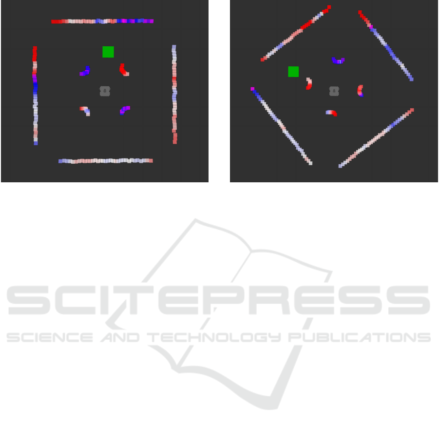
Figure 3: The rviz visualization shows the SHAP values for

Action 2 as the TurtleBot3 moves between the columns to-

ward the goal (represented by the green square), with the

TurtleBot3 positioned at the center of the image. The image

is oriented along the forward direction of the TurtleBot3.

Note that the corners of the outer walls appear missing

because the four columns obstruct the TurtleBot3’s view,

and the LiDAR only detects objects directly visible along

straight lines from its position.

LiDAR readings from these two columns to navigate

between them as we should expect, with the result be-

ing that the TurtleBot3 successfully moves towards

the goal.

A similar behavior is observed when the policy

has to turn the TurtleBot3 towards the goal when the

goal is currently located behind the TurtleBot3. Fig-

ure 4 shows the SHAP values for action 1, and the col-

umn straight ahead of the TurtleBot3 is colored blue,

which indicates that the policy uses the fact that there

is an obstacle straight ahead to make the linear veloc-

ity more negative.

4.2 Non-interpretable SHAP Values

Although we are, to some extent, able to interpret

some of the SHAP values in a way that makes sense

to a human, there are other situations where that is

difﬁcult. For both Figure 3 and Figure 4 discussed

above, the walls around the environment have what

seems to be quite noisy SHAP values. We can also

see the same in Figure 5, where the SHAP values

seem quite random and have a large magnitude for

the LiDAR readings at the walls for a single time step

at the beginning of each episode. To a human, these

SHAP values do not easily make sense. However, the

SHAP values indicate that these LiDAR readings are

important for the policy to navigate the environment.

We want to suggest that, since the policy uses the Li-

Figure 4: A visualization of the SHAP values for action 1

when TurtleBot3 is turning towards the goal behind it. Note

that the turtlebot3 is rotated approximately 45

◦

compared

to Figure 3 and that the visualizations are oriented with the

turtlebot3’s forward direction upwards, leading the environ-

ment to look rotated.

DAR readings from walls far away to navigate the en-

vironment, it is overﬁtting to the environment. We

hypothesize that the policy has memorized this par-

ticular environment and, in that way, knows how to

navigate it. If the policy used the LiDAR data for

obstacle avoidance instead, we would expect that the

closest obstacles would consistently have the largest

SHAP values. It is indeed quite likely that the pol-

icy has memorized the environment and thus is over-

ﬁtted to the environment since we have only trained

the policy using this environment. The authors in

(Cobbe et al., 2019) demonstrate how maze-solving

DRL agents can overﬁt to the training data even when

there are a remarkable number of different mazes in

the training data. Even though this is not directly ap-

plicable to our problem, it demonstrates the signiﬁ-

cant memorization capabilities of DRL agents, which

could indicate a likely overﬁtting in our agent as well.

Another problem is that the SHAP values can

change drastically between each time step. This could

make it very difﬁcult to interpret the SHAP values if

they are used to examine the system in real time.

4.3 Density-Based Clustering of SHAP

LiDAR Data

We will now look at the results from using the clus-

tering scheme described in Section 3.3 to condense

down the information in the SHAP visualizations

shown so far in the paper. Figure 6 shows the same

situation as in Figure 3, however with SHAP values

ICINCO 2024 - 21st International Conference on Informatics in Control, Automation and Robotics

338

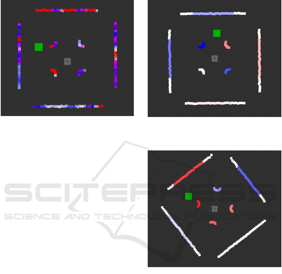
Figure 5: A visualization of the SHAP values for action

1 for the initial time step in an episode. This seemingly

random assignment of SHAP values with large magnitudes

to many LiDAR readings is consistent for the ﬁrst time step

in all episodes.

averaged across the clusters. We see the same ten-

dency with the left-forward column being blue and

the right-forward column being red, but with the clus-

tering scheme, it is much easier to read the visualiza-

tion. The SHAP values for the wall LiDAR readings

are also smoothed out. Figure 7 shows the same situa-

tion as Figure 4 after applying the clustering scheme.

Again, we see the same tendencies we discussed for

Figure 4. Finally, Figure 8 shows the same situation

as Figure 5 after applying the clustering scheme. This

plot looks much tidier now, and the clustering scheme

could, therefore, hide some of the complexity in the

agent’s decision-making. However, one would likely

need to create a balance between explanations that are

completely faithful to the model’s decision-making

and human-interpretable explanations.

5 CONCLUSION

In this paper, we have demonstrated the use of Shap-

ley Additive Explanations (SHAP) to interpret the

decision-making process of a DRL agent trained with

the SAC algorithm. The agent navigated a TurtleBot3

with a 360° LiDAR sensor through a simple obstacle

course in a simulated environment. By employing a

neural network with a convolutional layer to process

the LiDAR data, we aimed to leverage spatial correla-

tions between laser data points to improve navigation

performance.

Our results show that SHAP can provide valu-

able insights into the behavior of the DRL agent. We

Figure 6: This ﬁgure shows the same situation as in Fig-

ure 3, with the difference being that we instead show the

average SHAP values for each cluster of LiDAR points we

have found using DBSCAN.

Figure 7: This ﬁgure shows the same situation as in Fig-

ure 4, but after applying our SHAP value clustering scheme.

observed that the agent often made decisions based

on human-interpretable information, such as avoid-

ing obstacles detected by the LiDAR. However, there

were instances where the agent utilized non-intuitive

information, potentially indicating overﬁtting to the

speciﬁc training environment.

To visualize the SHAP values, we used them to

color a visualization of the LiDAR readings, showing

each reading’s contribution to the agent’s actions. To

address the noisy nature of SHAP values and their,

at times, drastic changes between time steps, we im-

plemented a density-based clustering approach using

DBSCAN. This clustering helped smooth the SHAP

visualizations, making them more interpretable for

Using Shapley Additive Explanations to Explain a Deep Reinforcement Learning Agent Controlling a Turtlebot3 for Autonomous

Navigation

339

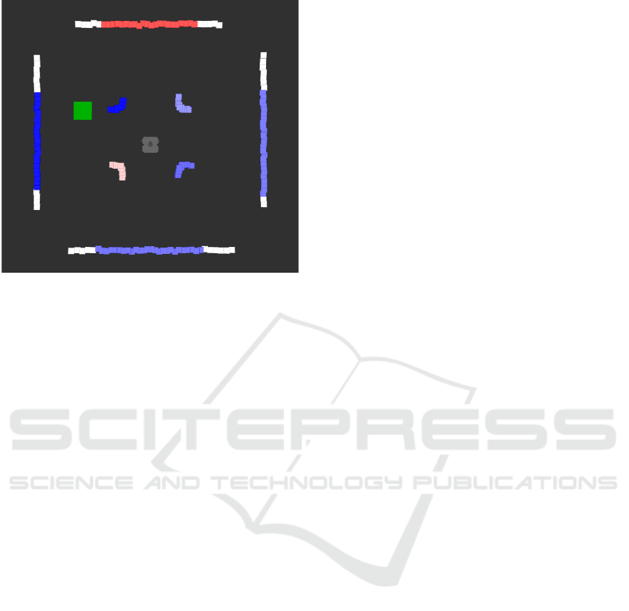
Figure 8: This ﬁgure shows the same situation as in Fig-

ure 5, but after applying our SHAP value clustering scheme.

real-time analysis.

Further work could, for instance, include under-

standing the reasons behind the high variability of the

SHAP values for minor changes in input data in this

environment. Another interesting possible future re-

search direction could be to see whether techniques

for reducing overﬁtting and improving generalization,

such as the domain randomization introduced in (To-

bin et al., 2017), could make the neural network pol-

icy prioritize obstacle avoidance instead of just rec-

ognizing its environment and in return changing the

SHAP values to a more human-interpretable distribu-

tion.

Overall, our ﬁndings suggest that while SHAP can

enhance the transparency of DRL agents, there are

still challenges in ensuring the interpretability of these

explanations.

ACKNOWLEDGEMENTS

The Research Council of Norway supported this

work through the EXAIGON project, project number

304843.

REFERENCES

Badia, A. P., Piot, B., Kapturowski, S., Sprechmann, P.,

Vitvitskyi, A., Guo, Z. D., and Blundell, C. (2020).

Agent57: Outperforming the atari human bench-

mark. In International conference on machine learn-

ing, pages 507–517. PMLR.

Bellotti, F., Lazzaroni, L., Capello, A., Cossu, M., De Glo-

ria, A., and Berta, R. (2023). Explaining a deep

reinforcement learning (DRL)-based automated driv-

ing agent in highway simulations. IEEE Access,

11:28522–28550.

Brunke, L., Greeff, M., Hall, A. W., Yuan, Z., Zhou, S.,

Panerati, J., and Schoellig, A. P. (2022). Safe learn-

ing in robotics: From learning-based control to safe

reinforcement learning. Annual Review of Control,

Robotics, and Autonomous Systems, 5:411–444.

Cimurs, R., Suh, I. H., and Lee, J. H. (2022). Goal-driven

autonomous exploration through deep reinforcement

learning. IEEE Robotics and Automation Letters,

7(2):730–737.

Cobbe, K., Klimov, O., Hesse, C., Kim, T., and Schul-

man, J. (2019). Quantifying generalization in rein-

forcement learning. In International conference on

machine learning, pages 1282–1289. PMLR.

Ester, M., Kriegel, H.-P., Sander, J., Xu, X., et al. (1996).

A density-based algorithm for discovering clusters in

large spatial databases with noise. In kdd, volume 96,

pages 226–231.

Gjærum, V. B., Str

umke, I., Løver, J., Miller, T., and

Lekkas, A. M. (2023). Model tree methods for ex-

plaining deep reinforcement learning agents in real-

time robotic applications. Neurocomputing, 515:133–

144.

Haarnoja, T., Zhou, A., Hartikainen, K., Tucker, G., Ha, S.,

Tan, J., Kumar, V., Zhu, H., Gupta, A., Abbeel, P.,

et al. (2018). Soft actor-critic algorithms and applica-

tions. arXiv preprint arXiv:1812.05905.

Koenig, N. and Howard, A. (2004). Design and use

paradigms for gazebo, an open-source multi-robot

simulator. In Proceedings of the IEEE/RSJ Interna-

tional Conference on Intelligent Robots and Systems

(IROS), volume 3, pages 2149–2154. IEEE.

Lundberg, S. M. and Lee, S.-I. (2017). A uniﬁed approach

to interpreting model predictions. Advances in neural

information processing systems, 30.

Molnar, C. (2022). Interpretable Machine Learning. 2 edi-

tion.

Quigley, M., Conley, K., Gerkey, B., Faust, J., Foote, T.,

Leibs, J., Wheeler, R., Ng, A. Y., et al. (2009). Ros: an

open-source robot operating system. In ICRA work-

shop on open source software, volume 3, page 5.

Kobe, Japan.

Rafﬁn, A., Hill, A., Gleave, A., Kanervisto, A., Ernes-

tus, M., and Dormann, N. (2021). Stable-baselines3:

Reliable reinforcement learning implementations. J.

Mach. Learn. Res., 22(268):1–8.

Remman, S. B., Str

umke, I., and Lekkas, A. M. (2022).

Causal versus marginal shapley values for robotic

lever manipulation controlled using deep reinforce-

ment learning. In 2022 American Control Conference

(ACC), pages 2683–2690. IEEE.

Shapley, L. S. (1952). A VALUE FOR N-PERSON GAMES.

Defense Technical Information Center.

Tobin, J., Fong, R., Ray, A., Schneider, J., Zaremba, W., and

Abbeel, P. (2017). Domain randomization for transfer-

ring deep neural networks from simulation to the real

world. In 2017 IEEE/RSJ international conference on

intelligent robots and systems (IROS), pages 23–30.

IEEE.

ICINCO 2024 - 21st International Conference on Informatics in Control, Automation and Robotics

340