Comparative Analysis of Brain Tumor Classification and Models

Based on VGG16

Yilin Chen

Faculty of Data Science, City University of Macao, Macao, China

Keywords: VGG16, Brain Tumor Diagnostics, Convolutional Neural Network.

Abstract: This study delves into the effectiveness of the Visual Geometry Group Network 16 (VGG16) convolutional

neural network (CNN) in the crucial task of classifying brain tumors, a pivotal endeavor aimed at enhancing

diagnostic accuracy and tailoring patient treatment in the field of oncology. Leveraging the renowned VGG16

model, celebrated for its deep architecture and robust feature extraction capabilities, this research seeks to

propel the accuracy of brain tumor diagnostics to new heights. Through a meticulously crafted methodology

encompassing comprehensive image preprocessing, meticulous optimization of the VGG16 model, and

meticulous comparison with other CNN models, the study meticulously evaluates crucial metrics such as

accuracy, sensitivity, and specificity. Drawing upon a rich dataset of brain tumor images for analysis, the

findings underscore VGG16's superior classification performance, highlighting its profound potential to

revolutionize medical imaging practices and elevate the standard of patient care in oncology. These

compelling results not only bolster the utilization of deep learning techniques in medical diagnostics but also

pave the way for future advancements in personalized healthcare methodologies.

1 INTRODUCTION

Brain cancer, a formidable adversary in oncology,

remains a leading cause of cancer-related morbidity

and mortality worldwide (Harachi, 2024). The

heterogeneity of brain tumors, with their complex

biological characteristics, presents a significant

challenge for accurate diagnosis and classification,

crucial for effective treatment planning (Xie, 2024).

The advent of Convolutional Neural Networks

(CNNs) has opened new vistas in medical image

analysis, offering a potential leap forward in the

precision of brain tumor classification (Irgolitsch,

2024). The significance of this research lies in

harnessing the power of CNNs, particularly the

Visual Geometry Group Network 16 (VGG16)

model, to improve the accuracy and efficiency of

brain tumor diagnosis, thereby contributing to

personalized medicine and better patient outcomes.

In the realm of medical image processing, CNNs

have emerged as a transformative force, particularly

in cancer diagnosis, including brain tumors. with

numerous studies demonstrating their efficacy in

classifying various types of cancers, including those

https://orcid.org/0009-0000-5833-2153

of the brain. In the domain of medical imaging,

particularly brain tumor classification, significant

strides have been made with the adoption of CNNs.

Research has evolved from traditional image

processing methods to advanced deep learning

models, with VGG16 emerging as a key player due to

its deep architecture and superior feature extraction

capabilitiesVGG16, a deep CNN architecture, has

been particularly noted for its success in image

recognition tasks due to its depth and robust feature

extraction capabilities(Jahannia, 2024). Previous

research has leveraged VGG16 for brain tumor

classification, achieving promising results that

underscore the model's potential in medical

applications(Khaliki, 2024). The VGG16

architecture, known for its depth and robust feature

extraction, has played a crucial role in this progress.

It has been effectively used for brain tumor

classification, showcasing the potential of deep

learning in medical applications. However, the

integration of CNNs in clinical workflows is still in

its infancy, with ongoing debates regarding model

interpretability, data privacy, and the need for large,

annotated datasets(Sachdeva, 2024). This study aims

652

Chen, Y.

Comparative Analysis of Brain Tumor Classiﬁcation and Models Based on VGG16.

DOI: 10.5220/0012961300004508

Paper published under CC license (CC BY-NC-ND 4.0)

In Proceedings of the 1st International Conference on Engineering Management, Information Technology and Intelligence (EMITI 2024), pages 652-658

ISBN: 978-989-758-713-9

to build upon the existing body of work, addressing

some of these challenges and pushing the boundaries

of what is currently achievable with CNN-based brain

tumor classification. The exploration of CNNs,

especially VGG16, in brain tumor classification not

only enhances diagnostic precision(Reddya, 2024)

but also paves the way for novel therapeutic

strategies. By accurately categorizing brain tumors,

clinicians can tailor treatments to individual patients,

thereby optimizing outcomes and minimizing adverse

effects(Balajee, 2024). Moreover, the integration of

CNNs into clinical decision-making processes

underscores the convergence of technology and

healthcare, promising a future where medical

interventions are more data-driven and patient-

specific(Yalamanchili, 2024). While the journey

toward fully integrating CNNs into routine clinical

practice is fraught with challenges, the potential

benefits in terms of improved diagnostic accuracy,

patient outcomes, and healthcare efficiency are

immense. The ongoing research and development in

this area are crucial steps toward realizing the full

potential of CNNs in medical imaging and oncology,

signifying a paradigm shift in how brain cancer is

diagnosed and treated(Rahman, 2024).

This study utilizes the VGG16 model to develop

a robust framework for brain cancer detection,

meticulously adjusting its parameters to gauge their

impact on model performance. Renowned for its deep

architecture and remarkable efficacy in feature

extraction, VGG16 plays a pivotal role in accurately

identifying various brain tumor types. To further

enhance the quality of the data, advanced image

preprocessing techniques are incorporated, thereby

augmenting the model's learning capabilities and

predictive accuracy. A comprehensive comparative

analysis with other CNN models is undertaken, with

a keen focus on key metrics such as accuracy,

sensitivity, and specificity in tumor classification.

Furthermore, the research evaluates VGG16's

scalability and consistency across diverse datasets

and operational scenarios, demonstrating its

adaptability in real-world settings. The results

unequivocally demonstrate that VGG16, coupled

with effective preprocessing techniques, surpasses

conventional models, representing a significant leap

forward in medical imaging. This advancement holds

both theoretical and practical implications, enhancing

diagnostic accuracy and potentially improving patient

treatment outcomes. Moreover, these findings

underscore the immense potential of deep learning in

medical diagnostics, paving the way for impactful

future research endeavors and clinical applications in

the realm of healthcare.

2 METHODOLOGIES

2.1 Dataset Description and

Preprocessing

The dataset used in this study is called the brain tumor

dataset and is derived from the Kaggle (Seif, 2024).

The dataset includes brain Magnetic Resonance

Imaging (MRI) scans obtained from patients with and

without brain malignancies. Each image acquire is

labeled with "Yes" or "No" to indicate the presence

or absence of the tumor. The aim here is to determine

the presence of tumors in the patient based on

magnetic resonance imaging. The training data set

contains 253 images, and before model development,

this study applies normalization techniques to

standardize the pixel values in the images.

Furthermore, this study applies the cropping function

to focus on regions of interest in brain MRI images,

which helps to reduce noise and irrelevant

information. Figure 1 shows some instances coming

from this dataset.

Figure 1: Part of the brain_tumor_dataset dataset

(Photo/Picture credit: Original).

2.2 Proposed Approach

Design and train CNN architectures specifically for

brain tumor detection, performing experiments using

different network architectures, regularization

techniques, and hyperparameters to optimize model

performance. This CNN model is a typical deep

learning model used for emotion classification tasks.

It contains multiple convolutional and pooling layers,

as well as fully connected and Dropout layers,

ultimately exporting a sigmoid-activated neuron for

the dichotomy task. The overall flow chart of the

model is shown in Figure 2.

Comparative Analysis of Brain Tumor Classiﬁcation and Models Based on VGG16

653

Figure 2: Flow diagram of the CNN network

(Photo/Picture

credit: Original).

The core construction of the model lies in its

clever use of multiple convolution layers and pooling

layers, which are connected and work together to

gradually extract various features from the input

images. These features start with the base edges and

textures and gradually upgrade to more complex and

higher-level feature representations. This hierarchical

feature extraction method enables the model to have

a deeper understanding of the image content, and lays

a solid foundation for the subsequent classification

task. After feature extraction, the model further

integrates and maps these features using the fully

connected layer. The fully connected layer transforms

the extracted features into a form corresponding to the

final output category by learning the weight and bias.

In this way, the model can predict the category of the

input image based on its features.

To prevent overfitting of the model during

training, this paper introduces the dropout layer. The

dropout layer is discarding some connections of

neurons randomly during training, so that the model

does not rely too much on some specific features or

weights to improve its generalization ability. At the

output end of the model, this study employs a neuron

with an s-type activation function. This neuron

transforms the model's predictions into a value

between 0 and 1, representing the probability that the

image belongs to a certain class. This probabilistic

output mode enables the model to show its prediction

results more intuitively and facilitates us to make

subsequent threshold setting and classification

decisions.

To optimize the training process of the model, this

study chooses the binary cross-entropy as the loss

function, which is well suited for scenarios with

dichotomous tasks. Meanwhile, this study also

adopted the Adam optimizer and set the learning rate

to 1e-4 to ensure that the model can be quickly and

stably converged to the optimal solution. This study

also performs a series of preprocessing steps before

the images enter the network. These steps include

resizing the images, normalizing them, and applying

data augmentation techniques. Through these

preprocessing measures, this study could not only

ensure the consistency and standardization of the

input data, but also improve the robustness of the

model, so that it can better cope with various complex

image changes and challenges.

2.2.1 Training Parameter Setting

During training, 50 training epochs were set and each

batch containing 32 samples to ensure that the model

was adequately learned and adapted to the data.

Meanwhile, to avoid overfitting of the model during

training, an early stopping strategy was used. When

the loss of the validation set does not significantly

improve over the five consecutive epochs, the

training ends early, thus preserving the performance

of the model at the best state. Before the training

started, this study performed a series of preprocessing

operations on the images. These operations include

adjusting the image size to meet the input

requirements of the model, performing normalization

processing to eliminate differences in brightness and

contrast between different images, and applying data

augmentation techniques to increase the diversity of

training samples and improve the robustness of the

model. The core part of the model consists of multiple

convolution layers and pooling layers. These

hierarchies enable automatic learning and extracting

key features in images, ranging from lower-level edge

and texture information to higher-level emotion-

related features. By passing and processing layer by

layer, the model can gradually deepen the

understanding of the image content. After feature

extraction, the model maps these features to the final

output category through a fully connected layer. The

fully connect layer transforms the prediction results

of the model into specific emotion classification

labels by learning and integrating feature information.

To prevent model overfitting, this study introduces

Dropout layers between the fully connected layers.

The Dropout layer randomly discards the connections

of some neurons during training, so that the model

does not rely too much on some specific features or

weights, thus improving its generalization ability.

During training, focus on loss and accuracy changes

in the training and validation sets. By monitoring

these indicators, this study could understand the

training state of the model and find and deal with

possible problems in time. Once the training is

complete, this study could use the model to classify

the new images emotionally and evaluate their

performance. The key to this classification method

lies in the rational design of the model structure and

EMITI 2024 - International Conference on Engineering Management, Information Technology and Intelligence

654

the training strategy. By continuously optimizing the

model parameters and the training process, this study

could improve the performance of the model in the

emotion classification task, so as to better understand

and analyze the information about the presence of

tumors in the image.

2.2.2 Loss Function

Loss function plays a crucial role in machine learning

and deep learning, measuring the difference between

model prediction results and actual labels, and is a

key indicator in the model optimization process.

Through the loss function, that can quantify the

performance of the model on the training set, and then

adjust the model parameters through the optimization

algorithm (such as gradient descent), so that the

model can better fit the data. Different tasks and

models may need to use different loss functions, and

common loss functions include mean square error

(MSE), cross-entropy, etc. Choosing the appropriate

loss function can help the model to better learn the

features of the data and improve the generalization

ability and accuracy of the model. Therefore, the loss

function can be regarded as an objective function

guiding the model learning and is an integral part of

the model training process. Here the binary crossover

loss function is used and the formula is as follows:

log( ( ))

(1 ) log(1 ( ))

ypy

Loss

ypy

=−

−−



(1)

For the binary label y, the value is not 0 or 1, while

p (y) indicates the probability that the output belongs

to the y label. As a key indicator of the prediction

effect of binary classification models, the binary

cross-entropy loss function plays a crucial role in

evaluating the model performance. In short, when the

label y is 1, if the p (y) value predicted by the model

is close to 1, it means that the prediction of the model

is highly consistent with the true label. At this time,

the value of the loss function should be close to 0,

indicating that the prediction effect of the model is

very good. On the other hand, if the p (y) value tends

to 0, that is, the model mistakenly predicts the sample

with label 1 to 0, the value of the loss function will

become very lase binary cross-entropy loss function

to effectively guide the model optimization, thus

improving the prediction accuracy of the binary

classification task.

3 RESULTS AND DISCUSSION

3.1 Confusion Matrix

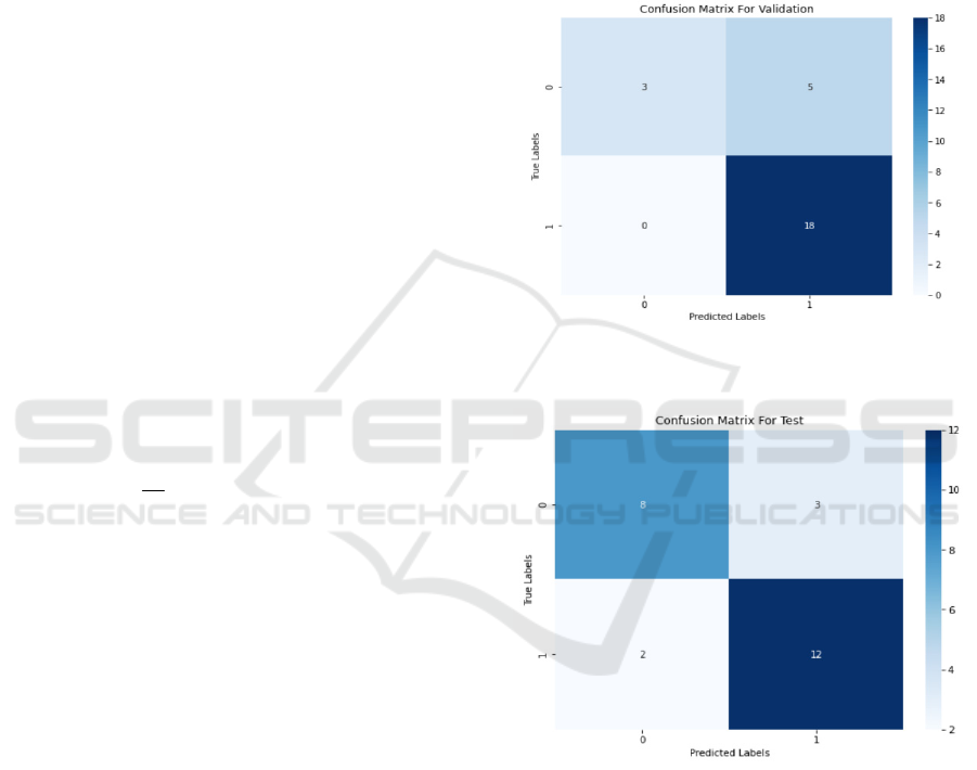
The confusion matrix represents the correspondence

between the predicted results and the true labels of the

model on the test set. The values of the confusion

matrix are slightly different compared to the

validation set, but the overall trend is similar.

Figure 3: Confusion matrix plot used for the validation

(Photo/Picture credit: Original).

Figure 4: Test the confusion matrix plot (Photo/Picture

credit: Original).

Figure 3 The model performs poorly on the

predicted category 0 (negative class), with a certain

number of false positive classes (misclassifying

negative classes as positive classes). The model

performed well on predictive category 1 (positive),

with most being correctly classified. The model

performs well on the validation set, but there is some

room for improvement in identifying negative

classes. This analysis helps us to understand how the

Comparative Analysis of Brain Tumor Classiﬁcation and Models Based on VGG16

655

model predicts on different categories, and thus guide

us to further adjustments and improvements.

Figure 4 The overall performance of the model on

the test set is relatively stable, like that on the

validation set. The number of false positive and false

negative classes increased slightly on the test set

compared to the validation set, but the overall

accuracy remained at a high level. Overall, the model

performed well on the test set, effectively

distinguishing between the two classes of samples,

but a small number of samples were still

misclassified. This analysis helps us to evaluate the

practical application of the model and provide a

reference for further improvement.

3.2 Plot of the Model Results

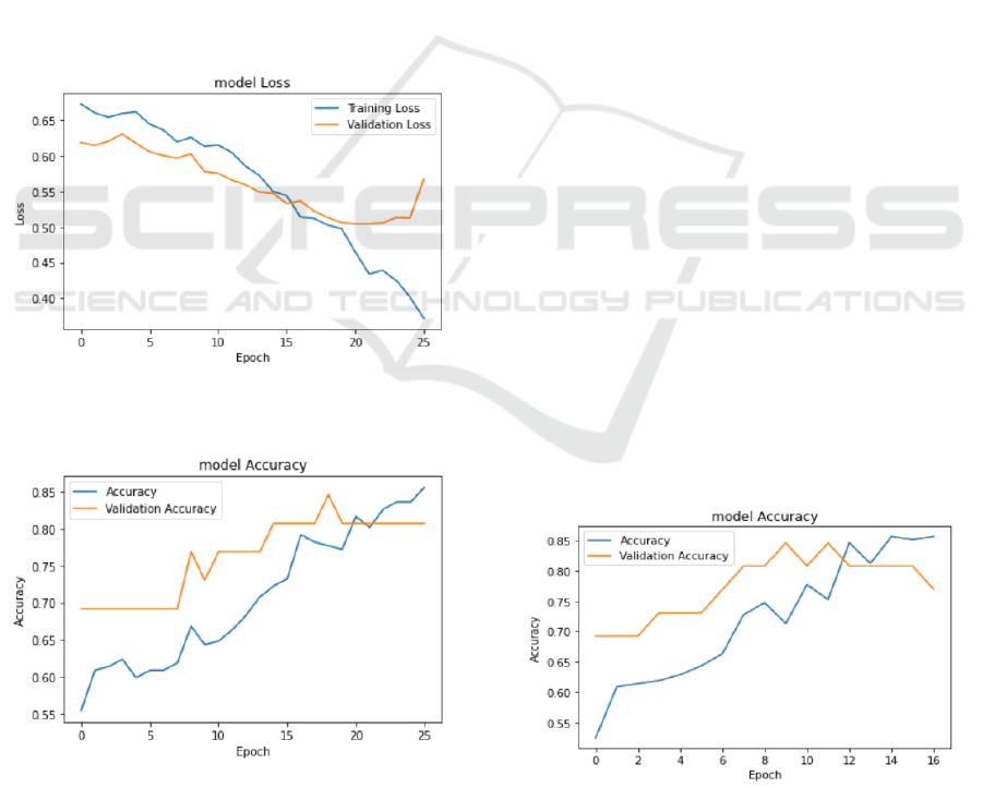
During the training process, with the increase of

epoch, the loss on the training set and the validation

set gradually decreases, and the accuracy gradually

improves.

Figure 5: Model loss function (Photo/Picture credit:

Original).

Figure 6: Model accuracy map (Photo/Picture credit:

Original).

Figure 5 With the increase of the epoch, the loss

value of the model gradually decreases in both the

training set and the validation set. This shows that the

model has gradually learned the characteristics of the

data during the training process and has made some

progress. However, it should be noted that the loss

values on the validation set do not always drop and

sometimes fluctuate, which may be caused by some

difficulties in the model during the training process or

noise from the data. Therefore, this study needs to

consider the performance on the training and

validation sets to comprehensively evaluate the

performance of the model.

Figure 6 shows that the accuracy of the model on

the training and validation sets increases with the

epochs. This shows that the model has gradually

learned the characteristics of the data during the

training process and has made some progress.

However, it should be noted that although the

accuracy of the model on the training set is constantly

increasing, the accuracy on the validation set is not

always increased, and sometimes it fluctuates or even

slightly decreases. This may be due to overfitting of

the model during training or noise from the data.

3.3 Adjust the Model Parameters

The original three convolution layers and pooling

layers were increased to three, and the number of

convolution kernels was adjusted to 64,128 and 256,

respectively, keeping the convolution kernel size at

(3,3) and the pooling layer size at (2,2). The number

of neurons in the fully connected layer adjusted the

original 128 neurons to 256.

With the increase of epoch, the accuracy of the

model on the training set was gradually improved,

from about 52.5% to about 85.6%. On the validation

set, the accuracy of the model showed a similar trend,

increasing from the initial ~ 69.2% to the final ~

80.8%, as shown in Figure 7.

Figure 7: Model accuracy chart (Photo/Picture credit:

Original).

EMITI 2024 - International Conference on Engineering Management, Information Technology and Intelligence

656

The model has certain generalization ability and can

perform well on unseen data. In later times, although

the model accuracy continued to improve on the

training set, the accuracy on the validation set began

to fluctuate and did not consistently improve. This

may be a sign of model overfitting and can adjust the

model structure or hyperparameters according to its

performance on the validation set to further improve

the model performance and generalization ability.

Possible adjustments include increasing data increase,

adjusting learning rate, adjusting network structure, etc.

3.4 Image Enhancement

Use ImageDataGenerator to perform image data

augmentation and create a data generator for the

training and validation sets. Specific data

enhancement operations include random rotation,

horizontal flip, vertical flip, random width, and height

offset, shear, and random scaling, etc. These

operations can increase the diversity of the data and

help to improve the generalization ability of the

model. The data generator of the training set uses the

data augmentation operation, while the data generator

of the validation set does not use the data

augmentation, maintaining the state of the original

data. In this way, the model can dynamically acquire

the enhanced data during training, further improving

the training effect, showing the partially enhanced

image as shown in Figure 8.

Figure 8: Image enhancement part of the image display

(Photo/Picture credit: Original).

3.5 VGG16 Model

The pre-trained VGG 16 model was used as the base

model, and several layers of global average pooling,

full connectivity and dropout layers were added to the

top, finally exporting a predicted layer of sigmoid

activation.

The pre-trained VGG 16 model was used, where

include_top=False represents the full connected layer

without the top, and input_shape= (128,128,3)

specifies the size of the input image as 128x128 pixels,

3 channels. All layers of VGG 16 were set to be

untrainable, that is, base_model.layers[0]. trainable =

False, so that the weights of these layers are not

updated during the training process, but only the

weights of the new layers. A global average pooling

layer GlobalAveragePooling2D () was added to the

output of the underlying model to transform the

feature map into a fixed length vector. Then comes a

fully connected layer, Dense (128, activation=

'relu',kernel_regularizer=regularizers.l2 (0.001)),

using the ReLU activation function and L2

regularization. A dropout layer Dropout (0.5) was

added to reduce overfitting. Finally, a Dense layer

was added as the output layer, using the sigmoid

activation function, for the deodorization task. The

model was compiled using the model. Compile

method, assigning the loss function as dichotomy

cross-entropy binary crossentropy, the optimizer as

Adam, with a learning rate of 1e-5, and the evaluation

index as accuracy.

EarlyStopping Used to stop training when the

validation set loss is no longer reduced to avoid

overfitting. The parameter monitor= 'val_loss'

represents the loss value of the monitored validation

set, patience=5 means that it stops training if the loss

is not reduced for five consecutive epoch validation

sets and restore_best_weights=True indicates the

weight restored to the best model when training is

stopped. ReduceLROnPlateau Is used to lower the

learning rate when the validation set loss is no longer

reduced to help the model converge better. The

parameter monitor= 'val_loss' represents the loss

value of the monitored validation set, factor=0.1

represents the factor by which the learning rate will

be reduced, patience=5 reduces the learning rate if the

loss of five consecutive epoch validation sets is not

reduced, and min _ lr = 1 e-7 represents the lower

limit of the learning rate. The model training was

performed using the model.fit method, assigning the

training set data generator train_generator and the

validation set data generator val_generator, training

20 epochs, and assigning the callback function as

[early_stopping, reduce _ lr]. The callback function

set like this can effectively control the training

process of the model, avoid overfitting, and achieve

better performance on the validation set.

Comparative Analysis of Brain Tumor Classiﬁcation and Models Based on VGG16

657

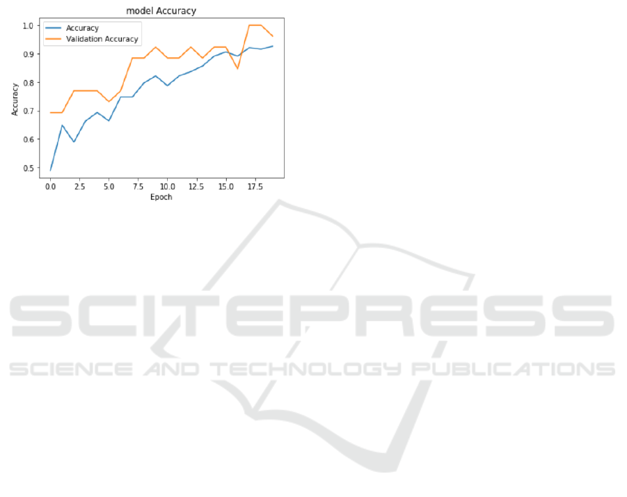
The accuracy of the model gradually improved during

the training process, finally achieving an accuracy of

about 92.6% on the training set and the highest

accuracy of about 96.2% on the validation set. This

shows that the model effectively learns the features of

the data during training and achieves good

performance on the validation set. As shown in Fig. 9.

Figure 9: Training accuracy of the VGG 16 model

(Photo/Picture credit: Original).

4 CONCLUSIONS

Firstly, this study embarked on a sentiment

classification project employing a CNN, commencing

with the utilization of a simple CNN model and

evaluating its performance on both training and

validation datasets. Subsequently, the focus shifted

towards leveraging the VGG16 model and fine-

tuning it, while integrating data augmentation

techniques to enhance the model's generalization

capabilities. For the simple CNN model, the observed

accuracy on the training and validation sets attained

approximately 85.6% and 80.8%, respectively.

Following the adoption of the VGG16 model and

fine-tuning approach, the accuracy on the training and

validation sets surged to around 92.6% and 96.2%,

respectively. Through the adjustment of the CNN

model's structure and parameters, alongside the fine-

tuning of the VGG16 model, endeavors were made to

bolster the model's performance. Noteworthy

callback functions such as Early Stopping and Reduce

learning rate On Plateau are deployed to monitor

model performance and dynamically adjust during

training iterations. While commendable results were

achieved with both the simple CNN and VGG16

models, superior performance was evident with the

VGG16 model, particularly in terms of accuracy on

the validation set.

REFERENCES

Balajee, A., Bharat, B., Mounica, N., & Mandava, S. (2024,

March). Brain tumour detection using deep learning. In

AIP Conference Proceedings, vol. 2966(1).

Harachi, M., Masui, K., Shimizu, E., Murakami, K.,

Onizuka, H., Muragaki, Y., ... & Shibata, N. (2024).

DNA hypomethylator phenotype reprograms

glutamatergic network in receptor tyrosine kinase gene-

mutated glioblastoma. Acta Neuropathologica

Communications, vol. 12(1), p: 40.

Irgolitsch, F., Huppé-Marcoux, F., Lesage, F., & Lefebvre,

J. (2024, March). Slice to volume registration using

neural networks for serial optical coherence

tomography of whole mouse brains. In Computational

Optical Imaging and Artificial Intelligence in

Biomedical Sciences, vol. 12857, pp: 107-115.

Jahannia, B., Ye, J., Altaleb, S., Peserico, N., Asadizanjani,

N., Heidari, E., ... & Dalir, H. (2024, March). Low-

latency full precision optical convolutional neural

network accelerator. In AI and Optical Data Sciences V,

vol. 12903, pp: 26-39.

Khaliki, M. Z., & Başarslan, M. S. (2024). Brain tumor

detection from images and comparison with transfer

learning methods and 3-layer CNN. Scientific Reports,

vol. 14(1), p: 2664.

Rahman, A. (2024). Brain tumour detection and

classification by using CNN (Master's thesis, Itä-

Suomen yliopisto).

Reddy, L. C. S., Elangovan, M., Vamsikrishna, M., &

Ravindra, C. (2024). Brain Tumor Detection and

Classification Using Deep Learning Models on MRI

Scans. EAI Endorsed Transactions on Pervasive Health

and Technology, vol. 10.

Sachdeva, J., Sharma, D., & Ahuja, C. K. (2024).

Comparative Analysis of Different Deep Convolutional

Neural Network Architectures for Classification of

Brain Tumor on Magnetic Resonance Images. Archives

of Computational Methods in Engineering, pp: 1-20.

Seif W., (2024). Brain Tumor Detection. https://www.

kaggle.com/code/seifwael123/brain-tumor-

classification-cnn-vgg16

Xie, H., Zhang, B., Xia, T., Cui, J., Pan, F., Li, Y., ... & Liu,

Y. (2024). Ezrin Thr567 phosphorylation participates in

mouse oocyte maturation, fertilization, and early

embryonic development. Fertilization, and Early

Embryonic Development.

Yalamanchili, S., Yenuga, P., Burla, N., Jonnadula, H., &

Bolem, S. C. (2024). MRI Brain Tumor Analysis on

Improved VGG-16 and Efficient NetB7 Models.

Journal of Image and Graphics, vol. 12(1).

EMITI 2024 - International Conference on Engineering Management, Information Technology and Intelligence

658