The Comparison of Diabetes Risk Prediction Accuracy Across

Different Models

Jing Yang

and Ruolan Zheng

School of Software Engineering, Shan Dong University, Jinan, 250101, China

School of Mathematics and Statistics, Nanjing University of Science and Technology, Nanjing, 210094, China

Keywords: Disease Prediction, Support Vector Machine, Random Forest, Multilayer Perceptron.

Abstract: The integration of machine learning technologies, particularly deep learning models, has significantly

advanced disease prediction within the healthcare industry. People have begun leveraging large-scale medical

data for research, combining various models aimed at enhancing the accuracy of medical disease prediction.

This study focuses on diabetes, a severe disease, and employs four different machine learning algorithms:

logistic regression, multilayer perceptron, support vector machine, and random forest. The author utilizes a

dataset obtained through direct questionnaire surveys of patients at the Sirhaj Diabetic Hospital in Bangladesh,

and conducts systematic data processing and visualization using the Python language to compare the strengths,

weaknesses, and effectiveness of these four models in disease prediction. This research aims to provide more

accurate and reliable tools for predicting the risk of diabetes in the healthcare field. Not only can this help

doctors better understand the health status of patients, but it can also provide crucial reference for personalized

treatment plans and preventive measures, thereby improving the cure rate of various major diseases.

1 INTRODUCTION

The healthcare sector has consistently been a frontier

for the remarkable success of deep learning

technology. The potent capabilities of deep learning

in pattern recognition and data analysis have

positioned it as a robust tool for addressing medical

challenges and enhancing patient care. In the realm of

healthcare, early prediction of severe diseases holds

paramount significance. Firstly, forecasting the future

progression of diseases aids in the timely

identification and preemptive intervention for

patients, thereby augmenting the chances of recovery.

Secondly, predictive models assist healthcare teams

in tailoring more precise and personalized medical

interventions, maximizing the efficacy of treatments.

Over the past few years, the area of disease

prediction has seen notable developments, with

numerous researchers achieving noteworthy

breakthroughs. In their investigation, Hosseininian

and colleagues (2024) employed a feature selection

approach grounded in ANOVA, or analysis of

variance to pinpoint the most pertinent features

https://orcid.org/0009-0004-6618-3257

https://orcid.org/0009-0008-4454-0371

concerning the prediction of Parkinson's illness by

means of using voice-based characteristics.

Subsequently, the Echo State Network (ESN) is

evaluated as a predictive model for this purpose.

Multiple models, encompassing the Echo State

Network, Decision trees, Support Vector Classifiers,

Random Forests, K-Nearest Neighbors, and Extreme

Gradient Boosting, were meticulously evaluated and

compared within the framework of the study. The

analysis of results highlights the exceptional

performance of the Echo State Network (ESN) among

the employed models (Hosseininian et al, 2024). Niu

et al. introduced an adaptive algorithm that improved

upon the conventional Grey Wolf Optimization

(GWO) with a sigmoid function, resulting in an

enhanced version of the Grey Wolf Optimization

algorithm for heart disease prediction (Niu et al,

2024). Wang et al. (2024) introduced an innovative

approach termed Hybrid Ordinal Prototype

Embedding (HOPE) in their research, aiming to

delineate the sequential advancement of Alzheimer's

disease for the prediction of mild cognitive

impairment progression. Mary studied supervised

Yang, J. and Zheng, R.

The Comparison of Diabetes Risk Prediction Accuracy Across Different Models.

DOI: 10.5220/0012968900004508

Paper published under CC license (CC BY-NC-ND 4.0)

In Proceedings of the 1st International Conference on Engineering Management, Information Technology and Intelligence (EMITI 2024), pages 697-703

ISBN: 978-989-758-713-9

697

machine learning algorithms for predicting heart

disease (Kanchan 2016). Frasca and colleagues

(2023) conducted an investigation utilizing the

dataset from the "Parkinson's Progression Markers

Initiative." Their study involved the development of a

deep learning model dedicated to discerning the

various stages of progression in Parkinson's disease.

The conclusive 3DCNN + LSTM model, trained and

assessed on MRI images, demonstrated exceptional

performance in accurately classifying the four distinct

levels of Parkinson's disease progression according to

the Hoehn and Yahr scale. This state-of-the-art model

achieved a macro-averaged One-Versus-Rest Area

Under the Curve (OVR AUC) of 91.90%.

However, the domain of disease prediction

confronts several difficulties and challenges. Issues

such as limited sample sizes for rare diseases leading

to reduced prediction accuracy, the complexity and

uncertainty inherent in disease prediction data, and

the inability of existing models to provide robust

predictions for unknown diseases pose significant

hurdles. Scholars have undertaken targeted research

efforts to address these challenges. The use of bio-

inspired optimization methods, such as the Genetic

Algorithm, Particle Swarm Optimization, and Whale

Optimization Algorithm, was examined by Dyoub et

al, for the purpose of selecting relevant features in

predicting chronic diseases. The primary aim of their

study was to improve the models' ability to anticipate

outcomes, simplify dimension of the data, and make

the resulting predictions more comprehensible and

applicable in a practical context (Dyoub and Letteri,

2023). Saba et al. (2024) introduced a novel

Continual Learning (CEL) model based on domain

adaptation and Elastic Weight Consolidation (EWC),

aiming to alleviate errors caused by catastrophic

forgetting in deep neural networks, such as LSTM, in

the context of incremental domain settings. In their

2019 study, Uddin and colleagues delved into the

predominant trends characterizing diverse categories

of supervised machine learning algorithms,

elucidating both their performance metrics and

practical applications in the realm of disease risk

prediction. Conclusions were drawn through a

comparative analysis. Dahiwade et al. (2019)

discovered that, in this general disease prediction,

considering individuals' lifestyle habits and

examination information enables accurate

forecasting. Patro et al. (2021) introduced an

innovative framework for predicting heart disease,

focusing on key risk factors and employing a variety

of classifiers, including Naïve Bayes (NB), Bayesian

Optimized Support Vector Machine (BO-SVM), K-

Nearest Neighbors (KNN), and Salp Swarm

Optimized Neural Network (SSA-NN). In their

investigation, the Convolutional Neural Network

(CNN) demonstrated a superior accuracy of 84.5% in

general disease prediction compared to the

performance of the KNN algorithm, or K-Nearest

Neighbors. The proposed optimization algorithm in

this framework aims to establish an effective

healthcare monitoring system for the early detection

of heart disease. This paper employs four algorithms

– Random Forest, Support Vector Machine (SVM),

Multilayer Perceptron (MLP), and logistic

regression-to foresee the likelihood of an individual

developing a specific illness. The accuracy of these

four algorithms will be compared to explore ways to

enhance the prediction capabilities for severe

diseases, consequently elevating the potential for

early detection and intervention. This introduction

sets the stage for a comprehensive exploration of

disease prediction methodologies and their potential

impact on healthcare outcomes.

2 METHODS

2.1 Data Source

These data are sourced from the UC Irvine Machine

Learning Repository. The data collection involved

direct questionnaire surveys with patients from Sylhet

Diabetes Hospital in Bangladesh, and it has received

approval from a doctor.

2.2 Indicator Selection and Description

Table 1 displays various symptoms and health

characteristics related to diabetes in the dataset used

for the study.

Table 1: Variable information.

Sympto

Introduction

Gende

1=Male, 0=Female

Pol

uria 1=Yes, 0=No

Pol

sia 1=Yes, 0=No

Sudden Weight Loss 1=Yes, 0=No

Weakness 1=Yes, 0=No

Polyphagia 1=Yes, 0=No

Genital Thrush 1=Yes, 0=No

Visual Blurrin 1=Yes, 0=No

Itchin

1=Yes, 0=No

Irritabilit

1=Yes, 0=No

Dela

ed Healin

1=Yes, 0=No

Partial Paresis 1=Yes, 0=No

Muscle Stiffness 1=Yes, 0=No

Obesity 1=Yes, 0=No

EMITI 2024 - International Conference on Engineering Management, Information Technology and Intelligence

698

2.3 Method Introduction

2.3.1 Data Processing

In this experiment, Python is used to systematically

process the data, employing the Pandas library to read

the dataset related to diabetes. The initial step

involves feature encoding, where the Label Encoder

is utilized to convert binary categorical features (such

as gender, presence of polyuria, etc.) into numerical

representations. For multi-categorical features, the

One Hot Encoder is used for independent encoding.

Subsequently, label encoding is performed using the

Label Encoder to convert categorical labels into

numerical format.

After that, the data set is separated into a training

and a test set, typically with an 80-20 ratio. Finally,

data standardization is conducted to normalize the

features, ensuring consistent scales across different

features, and enhancing the stability of the model

during training. This standardization is achieved

using the Standard Scaler function.

2.3.2 Support Vector Machine Model

Support Vector Machine is a supervised learning

algorithm suitable for binary classification problems.

Its main idea is to find an optimal hyperplane that

separates data points belonging to different types.

And then a linear kernel function is used to map the

data into a high-dimensional space, making it easier

to separate in the new space.

In the SVM model, the data was initially divided

into feature variables (X) and target variables (y).

Categorical features were processed using one-hot

encoding, while Label Encoder was employed to

convert the target variable into numerical form. The

data was divided into test and training sets in a two to

eight ratio. An SVM model was constructed with a

linear kernel function and a regularization parameter

C=1. Model performance was verified using 5-fold

cross-validation. The learning_curve function was

utilized to visualize the accuracy trends of the model

with different numbers of training samples.

2.3.3 Random Forest Model

The quarterly differential autoregressive moving

equilibrium model (SARIMA model) is an

improvement on the (ARIMA model), which is used

to transform non-smooth time series into smooth

periodic series. The model achieves the difference

and autoregressive moving average of the time series

by regression of the current and lagging values of the

dependent variable, as well as taking into account the

random error term. This transformation makes the

time series smoother and better able to capture

periodic features.

In the random forest model, categorical variables

were initially mapped to numerical representations.

Subsequently, the dataset was partitioned into feature

variables (X) and target variables (Y), and a random

forest classifier was employed for binary

classification. Model performance was assessed

through 5-fold cross-validation, followed by an

analysis of learning curves to examine the model's

ability at various training set sizes. The accuracy from

cross-validation was ultimately derived, and the

swerve of the model's training and validation

performance with increasing training data was

visualized using learning curve plots.

2.3.4 Multilayer Perceptron Model

A Multilayer Perceptron model is an artificial neural

network composed of multiple layers of neurons,

such as input, hidden and an output layer. Every

neuron has a connection with all neurons in the

preceding layer and is associated with weights and

biases. MLP captures complex relationships between

input features by learning these weights and biases.

In the MLP model, categorical variables were

initially converted into numerical representations

using Label Encoder. Subsequently, feature variables

(X) and target variables (y) were extracted. Following

this, Standard Scaler was applied to standardize the

features, ensuring uniform scales. The MLP model

was defined, comprising two hidden layers with 100

and 50 neurons, respectively, and a maximum

iteration limit set to 500. 5-fold cross-validation was

performed using Stratified K Fold, recording training,

and testing accuracies, as well as losses for each fold.

Finally, charts depicting the variation of training loss

and training/testing accuracies with the number of

iterations were generated to analyze the model's

performance.

2.3.5 Measurement

The Logistic Regression is a linear model which is the

main tool to solve binary classification problems. It

achieves the result by passing the weighted sum of

input features through a sigmoid function, mapping

the input to a probability range between 0 and 1,

facilitating classification.

In the logistic model, the data was initially

preprocessed and features were standardized.

Subsequently, the data was split into a training and a

testing set. This model was defined as a logistic

regression model with a linear layer, a Sigmoid

The Comparison of Diabetes Risk Prediction Accuracy Across Different Models

699

activation function, BCELoss loss function, and

trained for 500 epochs using the SGD optimizer.

Learning curves were employed to illustrate the

trends in training and testing accuracies. Ultimately,

the data of the model accuracy on the testing set was

reported.

3 RESULTS AND DISCUSSION

3.1 Analysis of Results

This study utilizes the pre-defined training set and

employs the Python language for visualizing the

output.

3.1.1 SVM Model Results

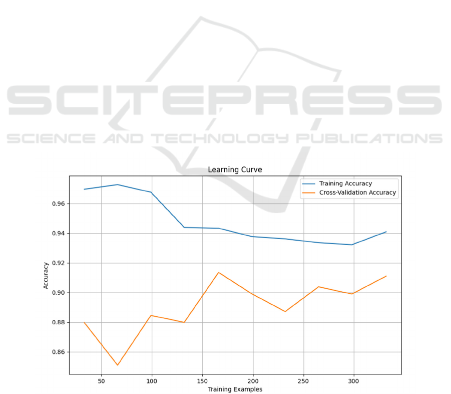
From Figure 1, with the increase in the number of

training samples, the Training Accuracy initially

experiences a slight decline before stabilizing. The

initial decrease may be attributed to overfitting noise

or local features when training on a small amount of

data. As the dataset grows, the model generalizes

better to overall features.

Test Accuracy exhibits fluctuations, but the

overall trend is a slow increase. The initial

fluctuations may arise from suboptimal performance

on specific validation sets during cross-validation

with a small dataset. With an increase in data, the

model's performance averages across different

validation sets, leading to a gradual rise in Test

Accuracy.

The trend of accuracy shows that the SVM has a

good performance on the training set without

significant overfitting. The gradual increase in Cross-

Validation Accuracy suggests that with more data, the

model performs better over a larger range and is likely

to generalize to unseen data. The model might benefit

from additional data to further enhance performance,

as the current sample size results in relatively high

fluctuations in Test Accuracy.

3.1.2 Random Forest Model Results

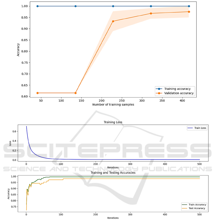
From Figure 2, Random Forest demonstrates strong

fitting capability, easily achieving perfect accuracy

on smaller training sets, resulting in a Training

Accuracy that remains stable at 1. The Test Accuracy

stabilizes initially, then rapidly increases with an

increase in training samples, eventually levelling off

at 97.3%. This suggests that the model starts

generalizing on larger samples and performs well on

the test set.

The strength of Random Forest lies in its fitting

ability to the data, but it is also prone to overfitting on

small datasets. Therefore, when using Random Forest

for predictive classification tasks, efforts should be

made to avoid overfitting, ensuring the model

maintains stable generalization on unseen data.

Figure 1: Support Vector Machine.

EMITI 2024 - International Conference on Engineering Management, Information Technology and Intelligence

700

Figure 2: Random Forest.

Figure 3: Multilayer Perceptron.

3.1.3 Multilayer Perceptron Model

From Figure 3, the training loss curve of the MLP

rapidly decreases during the initial stages of training

iterations before stabilizing, indicating that the model

has known the features of the data successfully. Both

training accuracy and test accuracy gradually increase

with an increase in the number of model iterations.

The test accuracy is a little lower than the training’s,

suggesting that the MLP performs well on both two

sets without exhibiting overfitting. The final model

achieves a test accuracy of 99.2%.

3.1.4 Logistic Regression Model Result

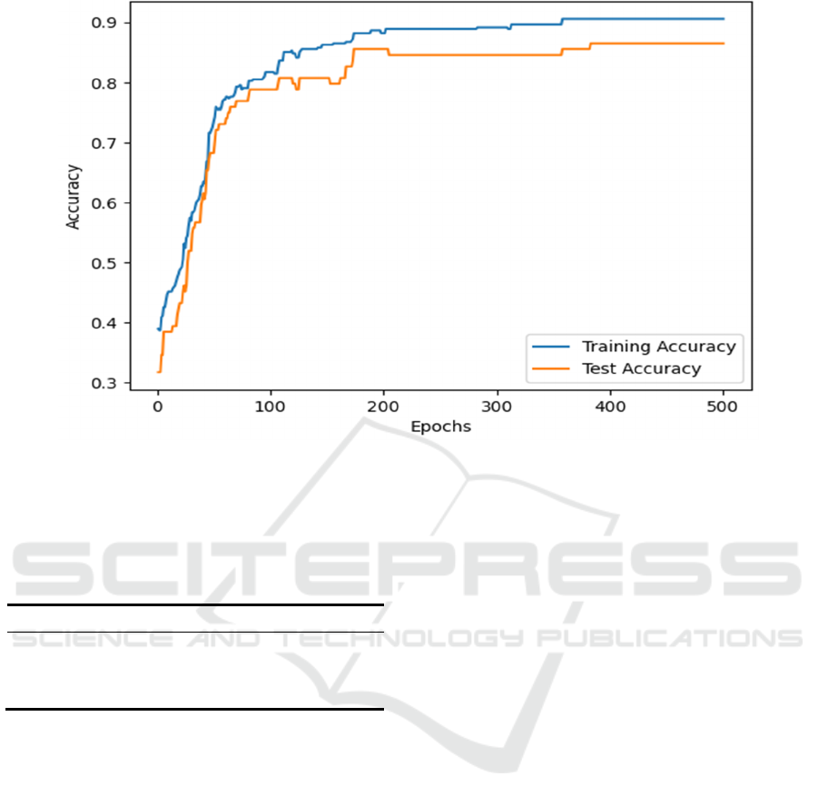
From Figure 4, the test accuracy figure is a little lower

than the trainings, and their accuracy curves exhibit a

similar upward trend with the number increase of

training epochs, eventually converging around a

stable value. This indicates that with an increase of

the model iterations, the accuracy of predicting

disease status significantly improves, ultimately

reaching 83.7%.

The Comparison of Diabetes Risk Prediction Accuracy Across Different Models

701

Figure 4: Logistic Regression.

3.2 The Comparison of Results

Table 2 shows the results of the four models.

Table 2: The Comparison of results.

Types of Models Test Accuracy

Support Vecto

Machine 0.911

Random Forest 0.973

Multilaye

Perceptron 0.992

istic Re

ression 0.837

Through comparing the performance of multiple

models, it was found that the Multilayer Perceptron

(MLP) excelled in this task, achieving an impressive

accuracy of 99.2%.

4 CONCLUSION

This study delved into the early diabetes prediction

domain, comparing the performance of various

models. It was observed that the Multilayer

Perceptron (MLP) exhibited outstanding performance

in this task, achieving 99.2% as the accuracy. Future

research could consider expanding the dataset to

validate the model's ability on a larger scale or

explore more sophisticated feature engineering to

improve the model's sensitivity to early diabetes

indicators or experiment with combinations of

different algorithms, potentially further improving

model performance.

AUTHORS CONTRIBUTION

All the authors contributed equally and their names

were listed in alphabetical order.

REFERENCES

Aslam, S., Rasool, A., Wu, H., Li, X., 2024. CEL: A

Continual Learning Model for Disease Outbreak

Prediction by Leveraging Domain Adaptation via

Elastic Weight Consolidation. Working paper.

Dahiwade, D., Patle, G., Meshram, E., 2019. March.

Designing disease prediction model using machine

learning approach. In 2019 3rd International

Conference on Computing Methodologies and

Communication (ICCMC). IEEE.

Dyoub, A., Letteri, I., 2023. Dataset Optimization for

Chronic Disease Prediction with Bio-Inspired Feature

Selection. Working paper.

Frasca, M., La Torre, D., Cutica, I., 2023. Combining

Convolution Neural Networks with Long-Short Time

Memory Layers to Predict Parkinson's Disease

Progression. Working paper.

Hosseininian, S. Z. S., Tajari, A., Ghalehnoie, M., Alfi, A.,

2024. Evaluating Echo State Network for Parkinson's

Disease Prediction using Voice Features. Working

paper.

EMITI 2024 - International Conference on Engineering Management, Information Technology and Intelligence

702

Kanchan, B. D., & Kishor, M. M., 2016. December. Study

of machine learning algorithms for special disease

prediction using principal of component analysis.

In 2016 international conference on global trends in

signal processing, information computing and

communication (ICGTSPICC). IEEE.

Niu, S., Zhou, Y., Li, Z., Huang, S., & Zhou, Y., 2024. An

Improved Grey Wolf Optimization Algorithm for Heart

Disease Prediction. Working paper.

Patro, S. P., Nayak, G. S., & Padhy, N., 2021. Heart disease

prediction by using novel optimization algorithm: A

supervised learning prospective. Informatics in

Medicine Unlocked, 26, 100696.

Uddin, S., Khan, A., Hossain, M. E., & Moni, M. A., 2019.

Comparing different supervised machine learning

algorithms for disease prediction. BMC medical

informatics and decision making, 19(1), 1-16.

Wang, C., Lei, Y., Chen, T., Zhang, J., Li, Y., Shan, H.,

2024. HOPE: Hybrid-Granularity Ordinal Prototype

Learning for Progression Prediction of Mild Cognitive

Impairment. Journal of Biomedical and Health

Informatics.

The Comparison of Diabetes Risk Prediction Accuracy Across Different Models

703