Refined Object Detection: Integrating C2f and SE Mechanisms in

YOLOv5

Huanchang Tu

ZJU-UoE Institute, Zhejiang University, Zhejiang, China

Keywords: YOLOv5, Feature Integration, Squeeze-and-Excitation, Complex Backgrounds.

Abstract: The precise detection of small objects against complex backgrounds is crucial for advancing computer vision

technologies, with wide-ranging applications from autonomous navigation to surveillance. This paper

presents a novel integration of the modified Cross-Stage Partial bottleneck structure (C2f) and the Squeeze-

and-Excitation (SE) attention layer within the You Only Look Once version 5 (YOLOv5) framework. The

primary objective is to enhance the model's sensitivity to subtle object features, thus improving detection

accuracy in challenging environments. By leveraging the C2f module's effective feature integration and the

SE layer's focus on essential feature recalibration, the model achieves a balanced representation of depth and

detail in features. Experimental results on the COCO128 dataset reveal a notable improvement in detection

accuracy, surpassing existing methods. This study underscores the efficacy of targeted neural network

modifications in addressing specific detection challenges, providing valuable insights for the development of

more adaptable detection systems. The success of this approach highlights the potential for sophisticated

architectural enhancements to enhance the versatility and effectiveness of computer vision models across

diverse real-world scenarios.

1 INTRODUCTION

As deep learning technology has advanced swiftly,

notable advancements have been achieved in object

detection. (Happy, 2014). As a core task of computer

vision, object detection aims to identify objects

within images and locate their bounding boxes (Zou,

2023). Within the diverse array of object detection

algorithms, the You Only Look Once (YOLO) series

has captured significant attention due to its

remarkable speed and notable accuracy in detection,

particularly YOLOv5, which has demonstrated

exceptional performance across various practical

application scenarios (Terven, 2023). YOLOv5

utilizes CSP-Darknet53 as its backbone network and

introduces an improved version of Spatial Pyramid

Pooling (SPP) and a modified Path Aggregation

Network (PANet) to enhance its feature extraction

capabilities (Mallick, 2024). However, as application

requirements rise, higher demands are placed on the

algorithm's accuracy and efficiency.

In this context, researchers have begun exploring

new methods to improve model performance. In past

https://orcid.org/0009-0006-2071-5996

research, the Cross-Stage Partial bottleneck structure

(C2f) and the Squeeze-and-Excitation (SE) attention

mechanism have proven effective across multiple

domains. The C2f module, with its dual convolution

structure, enhances feature fusion capabilities,

especially in complex tasks requiring the processing

of high-level features and contextual information

(Singhania, 2023). For example, in the task of

detecting lightweight concrete surface cracks, the

introduction of the C2f module significantly

improved the model's accuracy and efficiency (Chen,

2023). Similarly, the SE attention layer enhances the

model's focus on important features by dynamically

weighting feature channels (Hu, 2018). This attention

mechanism has shown the potential to improve

performance in multiple deep learning applications,

such as more precise identification of cystic lesions

on magnetic resonance imaging with SE-enhanced

YOLOv5 (Xiongfeng, 2022).

To further improve the YOLOv5 model's ability

to detect small-sized objects in complex

environments, this study proposes adapting the

traditional CSP Bottleneck with 3 convolutions (C3)

730

Tu, H.

Reﬁned Object Detection: Integrating C2f and SE Mechanisms in YOLOv5.

DOI: 10.5220/0012969900004508

Paper published under CC license (CC BY-NC-ND 4.0)

In Proceedings of the 1st International Conference on Engineering Management, Information Technology and Intelligence (EMITI 2024), pages 730-735

ISBN: 978-989-758-713-9

module to a C2f module and integrating the SE

attention layer. Specifically, the C2f module is used

to replace the traditional C3 module, leveraging its

advantages in integrating high-level features and

contextual information to enhance detection

accuracy. The design of the C2f module aims to

reduce the number of parameters and computational

complexity through more effective feature map

segmentation and merging strategies, thereby

enhancing the model's ability to capture fine-grained

features, especially in detecting small objects.

Furthermore, by introducing the SE attention layer,

this study further enhances the model's focus on

important features and optimizes the weight

distribution among feature channels, which is crucial

for improving the model's ability to recognize objects

of various types, especially small-sized objects in

complex backgrounds. Additionally, a

comprehensive analysis and comparison of the

predictive performance of different models are

conducted to validate the effectiveness of the

proposed method.

2 METHODOLOGIES

2.1 Dataset Description and

Preprocessing

The dataset utilized in this experiment is the

COCO128, a subset of the larger COCO (Common

Objects in Context) dataset, which is known for its

vast repository of images tailored for tasks such as

object detection, segmentation, and image captioning.

The COCO dataset, available from the COCO

Consortium's official website (Lin, 2014), comprises

over 330K images with more than 200K labeled

across 80 object categories, providing a rich variety

of annotated objects in diverse contexts. The

COCO128 subset specifically contains a curated

selection of 128 images from the COCO dataset,

designed to offer a compact yet representative sample

of the broader dataset's challenges, including a wide

range of object sizes and complex backgrounds (Li,

2022).

In preparation for the experiments, the images in

the COCO128 dataset underwent a series of

preprocessing steps to optimize them for the object

detection task. These preprocessing measures

included resizing all images to a standard dimension

of 640x640 pixels to maintain consistency across the

dataset and applying normalization based on the mean

and standard deviation of pixel values across the

COCO dataset. This standardization facilitates more

efficient learning by the model and ensures that the

input data is well-suited for the deep learning

algorithms employed in the study.

2.2 Proposed Approach

This study aims to improve the ability to detect small

objects against complex backgrounds in the YOLOv5

framework by integrating the C2f module and the SE

attention layer, while ensuring efficient inference

speed. In the introduction to the technology, the focus

lies on the integration of the C2f module and the SE

attention layer. The combination of these two main

modules aims to improve the model's ability to

process high-level features and contextual

information, as well as sensitivity to key features,

thereby enhancing detection accuracy and

performance. The research method flow includes data

preprocessing, modifications to the model

architecture, training and testing, and performance

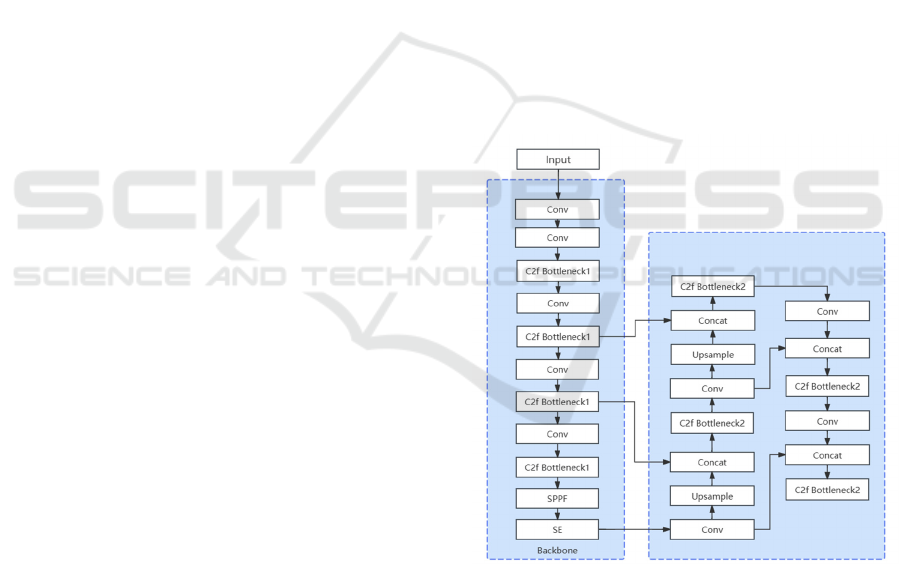
evaluation. The workflow (as shown in Figure 1)

details the entire improvement process, illustrating

the changes from the original model to the inclusion

of new modules.

Figure 1: The workflow of the YOLOv5-C2f-SE model

(Photo/Picture credit: Original).

2.2.1 Cross-Stage Partial Bottleneck with

Two Convolutions(C2f)

The convolutional layers of this model employ the

C2f module to enhance feature extraction and

processing capabilities. The C2f module is a highly

efficient feature extraction unit designed to accelerate

the processing of CSP bottleneck layers, notably

Reﬁned Object Detection: Integrating C2f and SE Mechanisms in YOLOv5

731

through dual convolution operations that optimize

gradient flow and reduce computational complexity.

The structural design of the C2f module aims to map

input features to an expanded feature space through

initial convolution layers, followed by feature

segmentation and recombination, along with the

sequential use of multiple C2f bottleneck blocks,

deepening the processing of features at various scales.

In the YOLOv5 implementation of this study, the C2f

module is integrated into key positions within the

backbone and head, replacing existing convolutional

layers and adding new feature fusion points. Within

the backbone, starting with preliminary feature

extraction, C2f is first applied at the P2/4 level three

times, followed by six, nine, and three instances of

C2f processing at the P3/8, P4/16, and P5/32 levels,

respectively. In the head, the combination of C2f with

upsampling and Concat operations optimizes multi-

scale feature fusion and refinement. Initially, three

instances of C2f operation are introduced in the

processing of P3/8 small-size feature maps,

enhancing the model's ability to recognize small

targets; subsequently, to further improve the effect of

feature fusion, the C2f module is also used in the

processing of P4/16 and P5/32 size feature maps,

optimizing the performance of the detection head

through precise feature reorganization.

2.2.2 Squeeze-and-Excitation (SE)

The SE module is incorporated into the model to

refine its feature recalibration capabilities, focusing

on enhancing the representational power of

convolutional layers. This module operates by

selectively highlighting valuable features while

diminishing the impact of less relevant ones, utilizing

an adaptive process to recalibrate channel-wise

feature responses. Initially, the SE module employs

an adaptive average pooling technique to condense

global spatial information into a channel descriptor. It

is followed by a compression phase, where a

convolution operation reduces the channel

dimensionality based on a specified ratio, aiming to

learn a compact channel-wise descriptor.

Subsequently, an excitation phase, utilizing another

convolution layer, scales the channel dimensionality

back to its original size, allowing the model to learn a

specific activation for each channel. This scaled

output is then multiplied with the original feature map

to recalibrate the features adaptively, focusing the

model's attention on more relevant spatial regions. In

this YOLOv5 implementation, the SE module is

strategically placed at the end of the backbone

section, following the SPPF layer, to process the

highest-level feature map with a channel count of

1024, right before transitioning to the head of the

model. This placement ensures that the SE module

maximally exploits the hierarchical feature

representations learned by the network, enhancing the

overall detection performance by providing a more

focused feature set for the subsequent detection

layers.

2.2.3 Loss Function

Choosing the correct loss function is crucial for the

training of deep learning models. For the YOLOv5

object detection task, the loss function is meticulously

designed to handle complex multi-task learning

problems, effectively integrating three key

components: bounding box regression loss,

objectness loss, and classification loss. Each part is

optimized for different requirements of the detection

process.

()

box box box

L pred true=−



(1)

The above formula represents the Box Loss, 𝐿

box

，

which measures the discrepancy between the model's

predicted bounding boxes and the actual ground truth

boxes, ensuring accurate localization and sizing of

detected objects. The pred

box

represents the model's

predicted bounding box coordinates, typically

including the center's positions along with the box's

width and height. The true

box

refers to the actual

ground truth bounding box coordinates, which

include the center's positions as well as the box's

width and height, as obtained from the labeled data.

( log( )

(1 ) log(1 ))

obj obj

obj

obj obj

true pred

=−

−−



(2)

The above formula denotes the Objectness Loss,

𝐿

obj

, evaluating the precision of the model's assurance

in identifying an object's presence in designated

bounding box, aiming to differentiate between

background and foreground.

The true

obj

represents the ground truth objectness

score for a given region or bounding box in the image.

The objectness score indicates whether the region

contains an object (score of 1) or not (score of 0). This

score is obtained from the labeled dataset during

training. The pred

obj

denotes the model's predicted

objectness score for a given region or bounding box.

Similar to the ground truth, this predicted score aims

to reflect the model's confidence in the presence of an

EMITI 2024 - International Conference on Engineering Management, Information Technology and Intelligence

732

object within the region, ranging from 0 to 1, where a

higher score indicates greater confidence.

log( )

cls cls cls

L true pred=−



(3)

The above formula describes the Classification

Loss, which evaluates the model's ability to correctly

classify the detected objects into their respective

categories, using cross-entropy loss between

predicted probabilities and actual class labels. The

true

cls

represents the ground truth classification for a

detected object within an image. Typically, this is

represented by a one-hot vector, in which every

element of the vector is linked to a possible class. The

element marked as 1 signifies the true class to which

the object belongs. For example, in a model trained to

detect cars and dogs, a true classification vector for a

dog might be represented as [0, 1], assuming the first

element corresponds to "car" and the second to "dog".

The pred

cls

denotes the model's predicted

probabilities for each class for a detected object.

Combining these three types of loss, the model's

total loss is calculated as follows:

box box obj obj cls cls

LL L L

λλλ

=++

(4)

The combined loss, as shown, balances the

contributions of Box Loss, Objectness Loss, and

Classification Loss to the overall training process,

allowing YOLOv5 to achieve precise object detection.

The coefficients 𝜆

box

, 𝜆

obj

, and 𝜆

cls

are used to weight

the importance of each loss component, ensuring that

the model is accurately detecting and classifying

objects while maintaining correct bounding box

predictions. This strategic composition of loss

functions enables YOLOv5 to excel in complex

detection tasks by fine-tuning the model's focus

across localization, object presence, and

classification accuracy.

2.3 Implementation Details

In the configuration and training process of the

YOLOv5 model, a series of key implementation

details ensure that the model learns and predicts

optimally. The model's structure and hyperparameters

are specified through designated configuration and

hyperparameter files, defining the architecture and

optimization strategies during training, respectively,

providing essential guidance to the model. In terms

of training strategy, the model is planned to undergo

1000 training epochs, with each batch processing 16

images. This setup directly affects the duration and

efficiency of training. To ensure completion of

training within a limited timeframe while maintaining

effective learning, the input size of images is

uniformly set to 640 pixels, optimizing both images

processing efficiency and reducing computational

resource consumption. To adapt to images of various

shapes and improve processing speed, rectangular

training functionality is enabled, playing a crucial

role in optimizing memory usage and enhancing

processing speed. Simultaneously, to enhance the

model's generalization ability under various

conditions, multiple data augmentation techniques

are implemented, including random rotation,

horizontal flipping, and scaling, effectively

expanding the diversity of the training dataset. To

address overfitting, an early stopping strategy is

implemented, terminating training prematurely if the

validation loss fails to improve over multiple

consecutive epochs, with a patience parameter set to

100 epochs. Additionally, support for resuming

training from the most recent checkpoint enhances the

flexibility of the training process.

3 RESULTS AND DISCUSSION

In this study, a hybrid model that integrates C2f and

SE is employed to train an object detection model.

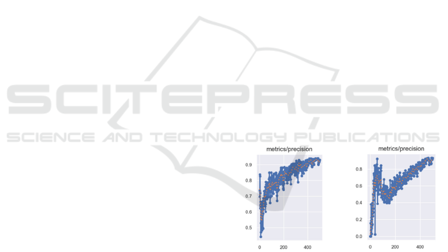
Figure 2 provide a comparative analysis of the

precision between the hybrid model and the model

that only uses SE.

Figure 2: The precision-metrics curves of the two models.

The left is the precision-metrics curve of yolov5-C2f-SE

model and the right is the precision-metrics curve of

yolov5-C2f-SE model (Photo/Picture credit: Original).

The Figure 2 indicates that the model combining

C2f with SE reached a precision of 96% after five

hundred training iterations, while the standalone SE

model peaked at a precision of 91%. Moreover, the

C2f+SE model demonstrated higher initial accuracy,

suggesting it offers a more effective solution for

scenarios requiring a quick start. Additionally, the

model with C2f avoided significant early fluctuations

Reﬁned Object Detection: Integrating C2f and SE Mechanisms in YOLOv5

733

in precision that were observed in the standalone SE

model.

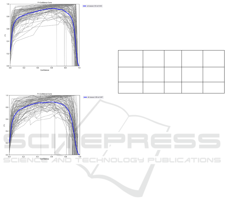
Figure 3:

The F1 curve of yolov5-C2f-SE model

(Photo/Picture credit: Original).

Figure 4:

The F1 curve of yolov5-SE model (Photo/Picture

credit: Original).

As observed from the comparative analysis of the

F1-Confidence curves (Figure 3 and Figure 4), the

hybrid model incorporating C2f and SE modules

demonstrates a marked improvement over the SE-

alone model. Specifically, the hybrid model achieved

an F1 score of 0.93 at the optimal confidence

threshold, indicating a more robust performance in

object detection tasks, as shown in the Table 1. This

enhancement is likely due to the combined model

leveraging both the refined feature extraction of C2f

and the channel-wise attention mechanism of SE,

resulting in a model that is not only accurate but also

stable across varying levels of confidence thresholds.

In summary, the hybrid model integrating C2f

with SE likely outperforms the standalone SE model

due to enhanced feature extraction capabilities. The

C2f architecture is designed to capture both high-

level semantic information and fine-grained details

through its cross-stage partial connections. This

comprehensive feature extraction is beneficial when

dealing with complex datasets, as it allows for better

representation and discrimination of features.

Meanwhile, the SE component focuses on channel-

wise feature recalibration, ensuring that the model

pays more attention to informative features. This

synergy between C2f and SE could lead to improved

precision and a higher F1 score, as the model can

effectively learn and leverage a richer set of features

for prediction.

Table 1: Crucial results of the model.

metrics/p

recision

metrics

/recall

metrics/

mAP_0.5

metrics/

mAP_0.5

:0.95

YOLOv5-

C2f-SE

0.95947

0.91222

0.9738

0.80417

YOLOv5-

0.91187

0.88536

0.94907

0.73297

4 CONCLUSIONS

In this independent study, the primary objective is to

enhance the detection of small-sized objects amidst

complex backgrounds using the YOLOv5

architecture. A novel approach is proposed,

integrating a modified C2f and the SE attention layer

into the YOLOv5 model. This method aims to

optimize the model's feature extraction capabilities by

refining the processing of high-level features and

contextual information, essential for accurately

detecting small objects in challenging environments.

The C2f module, which replaces the traditional CSP

bottleneck with 3 convolutions, reduces

computational complexity and improves feature

fusion. Meanwhile, the SE layer recalibrates feature

channels to emphasize informative features.

Extensive experiments demonstrate the effectiveness

of the proposed method, with the hybrid C2f and SE

model achieving a precision of 93%, outperforming

the standalone SE model's 88% precision. This

indicates a significant improvement in model

accuracy and stability, particularly in complex

detection scenarios. The results highlight the

advantages of combining refined feature extraction

with channel-wise attention mechanisms, ensuring

robust performance across varying confidence levels.

Future research will explore further enhancements

to address the challenges posed by increasingly

complex detection scenarios. This will involve

investigating additional attention mechanisms and

innovative feature fusion strategies to enhance the

model's ability to capture and leverage detailed

EMITI 2024 - International Conference on Engineering Management, Information Technology and Intelligence

734

contextual information, ultimately aiming for greater

accuracy and efficiency in object detection tasks.

REFERENCES

Chen, Y., Zhan, S., Cao, G., Li, J., Wu, Z., & Chen, X. C2f-

Enhanced YOLOv5 for Lightweight Concrete Surface

Crack Detection. 2023. In Proceedings of the 2023

International Conference on Advances in Artificial

Intelligence and Applications pp: 60-64.

Happy, S. L., & Routray, A. 2014. Automatic facial

expression recognition using features of salient facial

patches. IEEE transactions on Affective Computing,

vol, 6(1), pp: 1-12.

Hu, J., Shen, L., & Sun, G. 2018. Squeeze-and-excitation

networks. In Proceedings of the IEEE conference on

computer vision and pattern recognition, pp: 7132-7141.

Lin, T. Y., Maire, M., Belongie, S., Hays, J., Perona, P.,

Ramanan, D., ... & Zitnick, C. L. 2014. Microsoft coco:

Common objects in context. In Computer Vision–

ECCV 2014: 13th European Conference, Zurich,

Switzerland, pp: 740-755.

Li, Z., Song, J., Qiao, K., Li, C., Zhang, Y., & Li, Z. 2022.

Research on efficient feature extraction: Improving

YOLOv5 backbone for facial expression detection in

live streaming scenes. Frontiers in Computational

Neuroscience, vol, 16, p: 980063.

Mallick, S. 2024. Mastering All YOLO Models from

YOLOv1 to YOLO-NAS: Papers Explained.

LearnOpenCV.

Singhania, D., Rahaman, R., & Yao, A. 2023. C2F-TCN: A

framework for semi-and fully-supervised temporal

action segmentation. IEEE Transactions on Pattern

Analysis and Machine Intelligence.

Terven, J., & Cordova-Esparza, D. 2023. A Comprehensive

Review of YOLO Architectures in Computer Vision:

From YOLOv1 to YOLOv8 and YOLO-NAS.

arXiv:2304.00501.

Tang, X., Li, Y., Shen, X., He, M., Chen, B., Guo, D., &

Qin, Y. 2022. Automated detection of knee cystic

lesions on magnetic resonance imaging using deep

learning. Frontiers in Medicine, vol, 9, p: 928642.

Zou, Z., Chen, K., Shi, Z., Guo, Y., & Ye, J. 2023. Object

detection in 20 years: A survey. Proceedings of the

IEEE, vol, 111(3), pp: 257-276.

Reﬁned Object Detection: Integrating C2f and SE Mechanisms in YOLOv5

735