LSTM versus Transformers: A Practical Comparison of Deep Learning
Models for Trading Financial Instruments
Daniel K. Ruiru
1 a
, Nicolas Jouandeau
2 b
and Dickson Odhiambo
1 c
1
Starthmore University, Nairobi, Kenya
2
Universit
´
e Paris 8, Saint-Denis, France
Keywords:
Deep Learning, Recurrent Neural Networks, Long Short Term Memory (LSTM), Transformers.
Abstract:
Predicting stock prices is a difficult but important task of the financial market. Often two main methods
are used to predict these prices; fundamental and technical analysis. These methods are not without their
limitations which has led to the use of machine learning by analysts and investors as they try to gain an edge
in the market. In this paper, a comparison is made between recurrent neural networks and the Transformer
model in predicting five financial instruments; Gold, EURUSD, GBPUSD, S&P500 Index and CF Industries.
This comparison starts with base models of LSTM, Bidirectional LSTM and Transformers. From the initial
experiments, LSTM and Bidirectional LSTM have consistent results but with more trainable parameters. The
Transformer model then has few trainable parameters but has inconsistent results. To try and gain an edge from
their respective advantages, these models are combined. LSTM and Bidirectional LSTM are thus combined
with the Transformer model in different variations and then trained on the same financial instruments. The
best models are then trained on the larger datasets of the S&P500 index and CF Industries (1990-2024) and
their results are used to make a simple trading agent whose profit and loss margin (P/L) is compared to the
2024 Q1 returns of the S&P500 index.
1 INTRODUCTION
Predicting stock prices is a difficult task owing to the
ever changing and unpredictable nature of the finan-
cial market. Today, this goal of forecasting financial
markets has garnered a lot of attention from both aca-
demic and industrial practitioners who hope to pro-
vide provable answers for price outcomes. Many
methodologies have been suggested, often falling
within two major categories; technical and fundamen-
tal analysis (Kehinde et al., 2023). The former de-
fines techniques that evaluate investments based on
price patterns/trends while the latter focuses on the
intrinsic value of assets as well as the factors that
influence price outcomes (Krishnapriya and James,
2023). While somewhat effective, these methods still
face serious difficulties in providing solid answers or
even forecast of financial prices as exemplified by sig-
nificant fluctuations such as the 2008 financial crisis
which unfolded despite the existing technical and fun-
a
https://orcid.org/0000-0003-3197-8821
b
https://orcid.org/0000-0001-6902-4324
c
https://orcid.org/0000-0002-0968-5742
damental analyses. As such, a new phenomenon of
using machine learning algorithms to predict finan-
cial markets has been gaining popularity owing to the
success of these techniques in other domains. Ma-
chine learning methods use data to provide predic-
tions which academics and market traders/regulators
can use to forecast prices. Frameworks like Long
Short Term Memory Neural Networks (LSTMs) and
other Recurrent Neural Networks (RNNs) are of par-
ticular interest in the financial domains because of the
demonstrated superiority in dealing with time series
problems (Fischer and Krauss, 2018a). LSTM further
stands out as it has the ability to exploit and retain se-
quential data patterns over long periods of time. Re-
cently, this attribute of LSTM was enhanced through
the use of Transformers which shine in handling long
dependencies of input elements on top of enabling
parallel processing (Vaswani et al., 2017). Trans-
formers have thus become more effective in deal-
ing with tasks that use sequential data which explain
their popularity in Natural Language Processing do-
main. A similar challenge is exhibited by the finan-
cial markets as they pose a task in the sequential deci-
sion making problem domain which this paper tries to
Ruiru, D., Jouandeau, N. and Odhiambo, D.
LSTM versus Transformers: A Practical Comparison of Deep Learning Models for Trading Financial Instruments.
DOI: 10.5220/0012981100003837
Paper published under CC license (CC BY-NC-ND 4.0)
In Proceedings of the 16th Inter national Joint Conference on Computational Intelligence (IJCCI 2024), pages 543-549
ISBN: 978-989-758-721-4; ISSN: 2184-3236
Proceedings Copyright © 2024 by SCITEPRESS – Science and Technology Publications, Lda.
543

solve. This paper compares LSTM and Transformers
through their performance in predicting a variety of fi-
nancial instruments. Moreover, these two algorithms
are combined to try and yield a superior prediction
model.
The rest of the paper is organized as follows. Sec-
tion 2 outlines the Related Works, Section 3 briefly
discusses the Methodology, section 4 then reviews the
Experiments which is then followed by the Results
and Discussions in Section 5. Finally, Section 6 con-
cludes the study.
2 RELATED WORKS
Deep learning algorithms have shown great model-
ing prowess with non-linearity problems. LSTM and
Transformers can learn a lot of information from se-
quential data which explains their recent application
in complex time series modeling problems such as
stock/financial price prediction (Lin, 2023). The ap-
plication of these algorithms in the financial domain
are discussed below.
2.1 LSTM and Bidirectional LSTM
The LSTM model is actually a type of recurrent neu-
ral network (RNN) that was developed for modeling
sequential data. It uses gate units to manage the flow
of information which addresses the issues of gradi-
ent vanishing and explosion found in conventional
RNNs (Hochreiter and Schmidhuber, 1997). The ba-
sic LSTM structure shown in Figure 1 outlines a base
architecture that includes input gates, forget gates
and output gates. These gates selectively discard or
allow information flow through the network which
helps LSTM handle long sequences of information
and have better memory effect for any recurring pat-
terns. The input, forget and output gates are described
the following equations:
i
t
= σ(ω
i
[h
t−1
,x
t
] + b
i
) (1)
f
t
= σ(ω
f
[h
t−1
,x
t
] + b
f
) (2)
o
t
= σ(ω
o
[h
t−1
,x
t
] + b
o
) (3)
Where: i
t
is the input gate, f
t
is the forget gate, o
t
is
the output gate, σ is the sigmoid function, w
x
are the
weights of the respective gates, h
t−1
are the outputs
of the previous lstm block, x
t
is the input of the cur-
rent timestamp and b
x
are the biases for the respective
gates.
The mentioned attribute of LSTM make it ideal
for financial price modeling as it facilitates the ex-
ploration of long term dependencies found in mar-
ket prices. Many scholars and industrial practition-
Figure 1: Basic LSTM Structure.
ers have applied this basic structure in the financial
market. (Roondiwala et al., 2017); (Cao et al., 2019);
(Bao et al., 2017); (Fischer and Krauss, 2018b) all
used LSTM as a deep learning model for predicting
the financial market. In some cases, like that of (Bao
et al., 2017) they combined this base LSTM structure
with stacked auto encoders which yielded better re-
sults. In other cases, like that of (Siami-Namini et al.,
2019), bidirectional LSTM (BiLSTM) have been used
to increase the prediction performance by learning
long term dependencies across time steps of sequence
of data (time series) in both directions. This varia-
tion of LSTM is useful if a problem requires an RNN
to acquire information about an entire time series at
various iterations.
2.2 Transformers
On its part, Transformers are deep learning models
that also handle sequential data but unlike RNNs they
use a self-attention mechanism across their encoder-
decoder pair. At a high level, transformers can even
be seen as a sequence to sequence model but with an
encoder-decoder pair. The encoder is used to encode
the input sequence while the decoder produces the
output sequence (Vaswani et al., 2017); (Lin, 2023).
The self-attention mechanism found in this structure
then help to effectively pass information between the
encoder-decoder pair in both directions. Moreover,
self-attention also increases the encoding of the in-
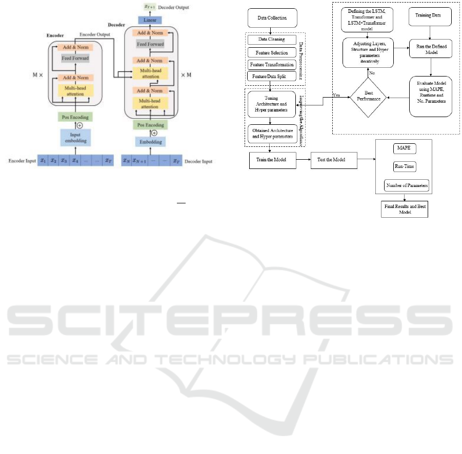
put sequence by the encoder. Figure 2 illustrates a
simple transformer architecture. The said attention
mechanism is facilitated by three vectors from the en-
coder’s input vectors. These three vectors are known
as Query (Q), Key (K) and Value (V) which are sim-
ply abstractions used to calculate transformers atten-
tion. In summary, these vectors are combined with a
softmax function to give the attention mechanism as
shown in equation 4. The role of the softmax func-
tion is to convert raw attention scores into probability
distributions.
NCTA 2024 - 16th International Conference on Neural Computation Theory and Applications
544

Figure 2: A Simple Transformer Architecture.
Attention(Q,K,V ) = so f tmax(QK
T
/
p
d
k
)V (4)
Today, Transformers have shown great efficiency
and versatility which have led to their extensive use
in many sequential decision making tasks. In partic-
ular, their ability to handle long sequence of data and
parallel process all the available data makes them su-
perior in capturing long range dependencies like those
in NLP and long term financial results/assessments.
3 METHODOLOGY
3.1 Defining the Problem
This paper uses LSTM and Transformers together
with their variants as reviewed in the literature re-
view. There was also an initial focus on the broadest
samples of these deep learning models, with modifi-
cations made to both the architecture and parameters.
The predictions made were done in four stages. First,
data collection, where a variety of datasets were ob-
tained to evaluate the proposed models’ performance.
Second, data pre-processing where the collected data
was enhanced to meet the requirements of the defined
models. Third, LSTM, Transformer and LSTM +
Transformer architecture and parameter optimization
to achieve the best results possible. Finally, predic-
tions were made based on trade simulations. Figure 3
summarizes this general road-map used in the experi-
ments of this paper.
3.2 LSTM and Transformer
To develop the final models used to predict financial
instruments, defining the problem also involved mod-
ifying the two base models LSTM and Transformer.
Figure 3: The General Road-Map.
To start with, a conventional unidirectional LSTM
and Bidirectional LSTM were used. These base mod-
els were then trained on the financial instruments with
their results recorded based on the evaluation met-
rics identified below (MAPE, Run-time and number
of parameters). Thereafter a basic transformer model
was implemented. This transformer model was then
trained on the financial instruments identified for this
study and the results were recorded based on the eval-
uation metrics.
3.3 Combining LSTM and
Transformers
Finally, the (best performing) LSTM model (based
on variation of layers) and Transformer model were
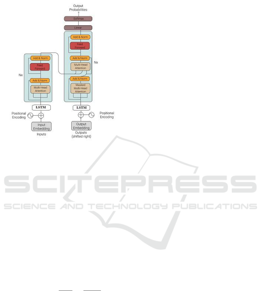
combined. In this case, the LSTM layer was added
just before the attention block of the Transformer as
illustrated in Figure 4. This resultant LSTM + Trans-
former model was then trained on the financial in-
struments and the results were recorded based on the
same evaluation metrics used in the previous models
training. This combination was the final step of the
experiments conducted.
3.3.1 Combining BiLSTM and Transformers
To cover the baseline model, Bidirectional LSTM was
also introduced. A similar structure was followed
with the combination of Bidirectional LSTM with
Transformer where the BiLSTM layer(s) was placed
before the attention block of the Transformer model.
LSTM versus Transformers: A Practical Comparison of Deep Learning Models for Trading Financial Instruments
545

Figure 4: Combining LSTM and Transformer.
3.4 Evaluation Metrics
Many evaluation metrics exist to assess the accuracy
of predicted results each with their own benefits. For
the experiments conducted, one conventional metrics
was used Means Absolute Percentage Error (MAPE)
owing to its ability to define the accuracy of forecast-
ing methods. MAPE outlines the average of the ab-
solute percentage errors of each entrant in a dataset
which then calculates how accurate a forecasted re-
sult is compared to an actual result (Jierula et al.,
2021). The choice of MAPE was also driven by its
ability to effectively analyze large sets of data such
as those found with the datasets used in this paper’s
experiments. Reviewing MAPE is also a straightfor-
ward process, with a 10 percent MAPE indicating a
10 percent deviation between the predicted value and
the actual value. Equation 5 summarizes MAPE.
MAPE(y, ˆy) =
100%
N
N−1
∑
i=0
|y
i
− ˆy
i
|
|y
i
|
(5)
In addition to MAPE, Run Time and Number of
Parameters used per model were used to assess the fi-
nal results. Generally, the prediction accuracy of any
model was not solely judged by the deviation from
the true value but also on the time it took to achieve
its predicted values (Run Time). Also, the number
of parameters used was a factor as they define the
resources used to run any given model. As such, in
an ideal case, a high accuracy of the predicted results
would be achieved with minimal run time and min-
imum number of parameters. As such, while trying
to achieve high performance/accuracy, the developed
model was expected to have minimal training param-
eters and run-time.
4 EXPERIMENTS
This section highlights two things; the datasets used
and the experiments done. The evaluations summa-
rized by this paper were based on five financial in-
struments - three forex pairs (Gold, GBPUSD, and
EURUSD); S&P500 (a stock market index) and CF
Industries Holdings stock prices (one of the stocks in
S&P500 index).
4.1 Data Selection and Preprocessing
The experiments done were based on large dataset for
all the five instruments. For the first 2 experiments
data from the 1st January 2013 to 2024 was used.
From experiment 3 to 5, only S&P500 and CF data
was used. The data used here was also larger, as it in-
cluded the period 1990 to 2024. In all the dataset, the
data collected was of the OHLC format (Open-High-
Low-Close). To get more stable analysis and results,
the daily time frame was used. The data was collected
from Yahoo Finance using the “yfinance” API. The
S&P500 and CF dataset was also manually obtained
from Stooq (stooq.com), an online resource that pro-
vides historical data for indices, stocks, bonds, forex
and other form of financial data.
4.2 Experiment 1
To get a benchmark for the experiments, the three
main models; LSTM, Bidirectional LSTM and Trans-
former were trained on the five financial instruments.
For the LSTM model, a base architecture with one
layer of 128 units was used, ultimately generating
73265 trainable parameters. A similar number of lay-
ers and units was used for the Bidirectional LSTM
(i.e. 1 layer with 128 units) and the total number
of trainable parameters ended being 146225. Finally,
the transformer model was based on a single trans-
former block which was then replicated to have the
needed number of blocks. For a start, 4 transformer
blocks were used resulting in 17205 trainable param-
eters. These three models were used to conduct the
first round of experiments with rankings being done
based on MAPE, Run-time and the number of param-
eters used to achieve their results. The results of this
first round (Experiment 1) are highlighted in the Re-
sults and Discussion section.
NCTA 2024 - 16th International Conference on Neural Computation Theory and Applications
546

4.3 Experiment 2
In an attempt to combine LSTM and Transformer to
yield a superior model, several variations of LSTM +
Transformers were developed and trained on the five
financial instruments. First, there was the base LSTM
with 1 layer of 128 units plus the basic four block
transformer model (here named LSTM128+TX).
Subsequently, LSTM with one layer of 64 units, 32
units and three layers of 128, 64 and 32 units were
combined with the transformer model (there naming
following a similar pattern as LSTM128+TX). Sim-
ilarly, the Bidirectional LSTM was combined with
the transformer model with a familiar naming pattern:
BiLSTM128+TX, BiLSTM64+TX, BiLSTM32+TX
and BiLSTMAll+TX. These combinations and the
number of trainable parameters used are summarized
below in Table 1.
Table 1: Combined Models and Number of Parameters.
Model No. Parameters
LSTMAll + TX 833394
LSTM128 + TX 1523346
LSTM64 + TX 651474
LSTM32 + TX 301554
BiLSTMAll + TX 2083794
BiLSTM128 + TX 3430930
BiLSTM64 + TX 1392274
BiLSTM32 + TX 618706
These combinations of LSTM/BiLSTM and
Transformer were then ranked based on their MAPE,
Run-time and number of parameters. The results of
these tests (Experiment 2) are highlighted in the Re-
sults and Discussion section.
4.4 Experiment 3
For the third experiment, the three best models, (ei-
ther base model or combination models) were then
used to predict the S&P500 index and CF industries.
Prior to experiment 3, a quick summary of the best
performing models, based on experiment 1 and 2 was
done to help identify the 3 best models.
4.5 Experiment 4 and 5
In this final round of experiments, the two financial
instruments (S&P500 and CF Industries) were pre-
dicted with the three best models from experiment
3. Also, this final round of experiment saw an in-
depth review of the prediction of the CF industries
prediction by the best model. Thereafter, this pre-
diction/forecast was compared with the returns of in-
vesting in the S&P500 index in the last month of the
dataset used. In all, this final test was to see whether
the best model from these experiments would chal-
lenge the returns of the S&P500 index in 2024.
5 RESULTS AND DISCUSSIONS
Table 2: Sample of Experiment 1 Results - Gold.
Experiment 1: Gold
Model MAPE Run-Time No. Para
LSTM128 0.0143 84.27s 73265
BiLSTM128 0.0134 51.50s 146225
TX 0.0134 150.24s 17205
The Tables 2 and 3 highlight a sample of the results of
the first and second experiment where all models were
tested with the five financial instruments. From ex-
periment 1, one results that stood out was the lack of
consistency in the results of the Transformer model.
Over a run of multiple training iterations including
some of the same parameters and financial instru-
ments, the Transformer model failed to have similar
or comparable results. Moreover, the first experiment
also broke a notion that was held at the start of the
tests that the fewer number of parameters in the Trans-
former model would results in a shorter run-time. Sur-
prisingly, the Transformer model regularly took the
longest time to run the training but yielded compet-
itive results. On their part, the LSTM and Bidirec-
tional LSTM were more consistent with their results,
including have comparable outcomes in multiple iter-
ations of same financial instruments.
Table 3: Sample of Experiment 2 Results - Gold.
Experiment 2: Gold
Model MAPE Run-Tim No.Para
LSTMAll+TX 0.0140 351.37s 833394
LSTM128+TX 0.0155 333.65s 1523346
LSTM64+TX 0.0183 213.63s 651474
LSTM32+TX 0.0168 151.58s 301554
BiLSTMAll+TX 0.0147 604.48s 2083794
BiLSTM128+TX 0.0142 518.57s 3430930
BiLSTM64+TX 0.0199 280.53s 1392274
BiLSTM32+TX 0.0186 221.33s 618706
On experiment 2, the combination of
LSTM/BiLSTM with Transformer model pro-
duced models that had consistent results. It was
much easier to replicate a prediction with them which
validated their use. Of note was the Run-time of the
BiLSTMAll+TX and BiLSTM128+TX which was
often the longest in any of the categories tested. This
outcome is easily attributed to the total number of
LSTM versus Transformers: A Practical Comparison of Deep Learning Models for Trading Financial Instruments
547

trainable parameters used; 2083794 and 3430930
respectively.
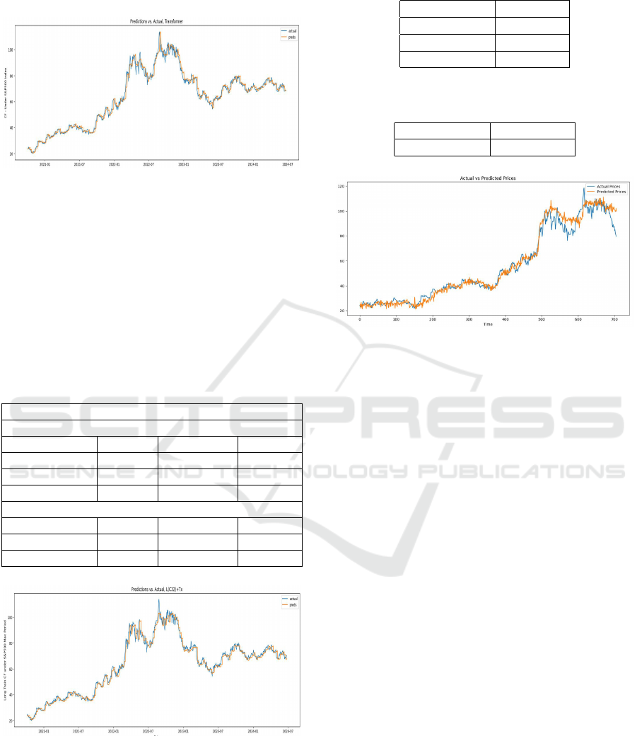
Figure 5: Sample Experiment 2 - LSTMAll+TX.
The ranking done in experiment three saw, 3 mod-
els emerge as favorite based on their leading perfor-
mance in MAPE, Run-time and number of training
parameters (fewer being better). The three models
were LSTM with 1 layer of 32 units combined with
Transformer (LSTM32 + TX), the base Transformer
model (TX) and the base Bidirectional LSTM (with
1 layer of 128 units). These three were then used in
experiment 4 and 5 where tables 4 and 5 summarizes
the overall results.
Table 4: Sample of Experiment 4 Results - S&P500 Index.
Experiment 4: S&P500 Index
Under 75 epochs
Model MAPE Run-Tim No.Para
LSTM32+TX 0.0149 949.04955s 301554
TX 0.0207 553.503s 17205
Bi-LSTM 0.01509 350.8049s 146225
Under 300 epcohs
LSTM32+Tx 0.01964 986.7037s 301554
TX 0.02699 547.1845s 17205
Bi-LSTM 0.01334 543.042s 146225
Figure 6: Experiment 4 - Prediction of CF Industries.
From these results it is clear that the combined
model of LSTM and Transformer outperforms all the
other models in predicting CF Industries. This obser-
vation further led to the development of a basic trad-
ing agent that used the LSTM32+TX model. While
its performance changed rapidly, the best, positive re-
Table 5: Experiment 5 - Predicting CF Industries.
Model Accuracy
LSTM32+Tx 95.9154%
TX 93.2079%
Bi-LSTM 91.6369%
Table 6: Experiment 5 - Trading CF Industries with
LSTM32+TX Based Agent.
Model-Agent %Change
LSTM32+Tx 0.012-0.768
Figure 7: Visualizing CF Industries Trading.
sults (profitable P/L) ranged between 1.2 percent to
7.68 percent return on initial investment which is not
bad compared to the S&P500 index 2024(Q1) returns
of about 15 percent (Curvo, 2024); (Speights, 2024).
Therefore, with good risk management, a potential
trader could get good returns by combining funda-
mental and technical analysis with an LSTM + Trans-
former model.
6 CONCLUSIONS
In this paper, LSTM, Bidirectional LSTM and Trans-
former models were compared in predicting five fi-
nancial instruments. From an initial forecast, three
best performing models were used to further pre-
dict S&P500 index and CF Industries based on large
datasets. The best model was then tested as a trading
agent model which yielded good results. This agent
however had erratic results which is solid ground for
future works, as one tries to stabilise the trading out-
comes. In future works, one can try to stabilize the
trading results by either adding more trading heuris-
tic, modifying the base model or changing the speci-
fication of the trading environment.
NCTA 2024 - 16th International Conference on Neural Computation Theory and Applications
548

REFERENCES
Bao, W., Yue, J., and Rao, Y. (2017). A deep learning
framework for financial time series using stacked au-
toencoders and long-short term memory. PloS one,
12(7):e0180944.
Cao, J., Li, Z., and Li, J. (2019). Financial time series fore-
casting model based on ceemdan and lstm. Physica A:
Statistical mechanics and its applications, 519:127–
139.
Curvo (2024). S&P 500: historical performance from 1992
to 2024. [Online; accessed 9. Jul. 2024].
Fischer, T. and Krauss, C. (2018a). Deep learning with long
short-term memory networks for financial market pre-
dictions. European journal of operational research,
270(2):654–669.
Fischer, T. and Krauss, C. (2018b). Deep learning with long
short-term memory networks for financial market pre-
dictions. Eur. J. Oper. Res., 270(2):654–669.
Hochreiter, S. and Schmidhuber, J. (1997). Long short-term
memory. Neural computation, 9(8):1735–1780.
Jierula, A., Wang, S., Oh, T.-M., and Wang, P. (2021). Study
on accuracy metrics for evaluating the predictions of
damage locations in deep piles using artificial neural
networks with acoustic emission data. Applied Sci-
ences, 11(5):2314.
Kehinde, T., Chan, F. T., and Chung, S. H. (2023). Scien-
tometric review and analysis of recent approaches to
stock market forecasting: Two decades survey. Expert
Systems with Applications, 213:119299.
Krishnapriya, C. and James, A. (2023). A survey on stock
market prediction techniques. In 2023 International
Conference on Power, Instrumentation, Control and
Computing (PICC), pages 1–6. IEEE.
Lin, Z. (2023). Comparative study of lstm and transformer
for a-share stock price prediction. In 2023 2nd Inter-
national Conference on Artificial Intelligence, Inter-
net and Digital Economy (ICAID 2023), pages 72–82.
Atlantis Press.
Roondiwala, M., Patel, H., Varma, S., et al. (2017). Predict-
ing stock prices using lstm. International Journal of
Science and Research (IJSR), 6(4):1754–1756.
Siami-Namini, S., Tavakoli, N., and Namin, A. S. (2019).
A comparative analysis of forecasting financial time
series using arima, lstm, and bilstm. arXiv preprint
arXiv:1911.09512.
Speights, K. (2024). The S&P 500 Jumped Nearly 15% in
the First Half of 2024. Here’s What History Says It
Could Do in the Second Half of the Year. [Online;
accessed 9. Jul. 2024].
Vaswani, A., Shazeer, N., Parmar, N., Uszkoreit, J., Jones,
L., Gomez, A. N., Kaiser, Ł., and Polosukhin, I.
(2017). Attention is all you need. Advances in neural
information processing systems, 30.
LSTM versus Transformers: A Practical Comparison of Deep Learning Models for Trading Financial Instruments
549