Unscented Transform-Based Pure Pursuit Path-Tracking Algorithm

Under Uncertainty

Chinnawut Nantabut

The Sirindhorn International Thai-German Graduate School of Engineering, King Mongkut’s University of Technology

North Bangkok, 1518 Pracharat 1 Road, Wongsawang, Bangsue, Bangkok, Thailand

Keywords:

Autonomous Vehicles, Automated Driving, Path-Tracking Algorithm, Uncertainty.

Abstract:

Automated driving has become more and more popular due to its potential to eliminate road accidents by taking

over driving tasks from humans. One of the remaining challenges is to follow a planned path autonomously,

especially when uncertainties in self-localizing or understanding the surroundings can inﬂuence the decisions

made by autonomous vehicles, such as calculating how much they need to steer to minimize tracking errors.

In this paper, a modiﬁed geometric pure pursuit path-tracking algorithm is proposed, taking into consideration

such uncertainties using the unscented transform. The algorithm is tested through simulations for typical road

geometries, such as straight and circular lines.

1 INTRODUCTION

Signiﬁcant research in the ﬁeld of autonomous vehi-

cles seeks to reduce injuries and fatalities by fully re-

placing human decision-making in driving. Despite

the recent surge in the popularity of self-driving cars,

research into tracking algorithms - where vehicles at-

tempt to stay close to a desired reference path - has

been ongoing for decades.

Several approaches, including geometry-based,

robust, optimization-based, and AI-based algorithms,

are commonly employed to address this challenge

(Rokonuzzaman et al., 2021). Geometry-based algo-

rithms, such as pure pursuit controllers, remain pop-

ular due to their simplicity. These algorithms rely

solely on geometric information from the vehicle and

its current position relative to the tracked path, al-

lowing timely decisions to handle potential hazards.

Recent tests have applied this algorithm in driver as-

sistance systems (Wang et al., 2017) and agricultural

ﬁeld tests (Qiang et al., 2021).

However, geometry-based algorithms are most ef-

fective when vehicle limitations are not exceeded,

such as during highway driving or aggressive steering

maneuvers, as demonstrated by (Nan et al., 2021). In

scenarios where vehicle constraints are not fulﬁlled,

optimization-based algorithms like Linear Quadratic

Regulator (LQR), Model Predictive Control (MPC),

https://orcid.org/0000-0002-5767-6023

and AI-based methods - such as neural networks that

can model vehicle behavior more precisely - are of-

ten better suited. In typical cases, such as low-speed

urban trafﬁc, a kinematic bicycle model combined

with geometric-based algorithms is sufﬁcient. For in-

stance, (Lee and Yim, 2023) showed that pure pursuit

algorithms can achieve similar tracking performance

to LQR and MPC in low-friction conditions.

Though considered a traditional method, the pure

pursuit algorithm continues to attract research inter-

est. Much of the work explores optimal ways to

determine the look-ahead distance, measured from

the vehicle’s rear axle to the reference path. Re-

cent studies have also incorporated techniques from

other tracking algorithms into pure pursuit. For exam-

ple, (Li et al., 2023) integrated adaptive pure pursuit

to enhance path planning in cluttered environments.

These adaptations incorporate principles from more

advanced tracking algorithms, helping to optimize the

look-ahead distance.

In AI-based methods, (Joglekar et al., 2022) ap-

plied deep reinforcement learning (DRL) to skid-

steered vehicles, enhancing adaptation in nonlinear

off-road scenarios compared to MPC.

Regarding optimization techniques, evolutionary

algorithms are often used. For example, (Wang et al.,

2020) employed the Salp Swarm Algorithm (SSA) to

optimize the look-ahead distance for improved track-

ing, while (Wu et al., 2021) used Particle Swarm Opti-

mization (PSO) to adjust preview distances based on

182

Nantabut, C.

Unscented Transform-Based Pure Pursuit Path-Tracking Algorithm Under Uncertainty.

DOI: 10.5220/0012981400003822

Paper published under CC license (CC BY-NC-ND 4.0)

In Proceedings of the 21st International Conference on Informatics in Control, Automation and Robotics (ICINCO 2024) - Volume 2, pages 182-189

ISBN: 978-989-758-717-7; ISSN: 2184-2809

vehicle speed and track curvature. Similarly, (Yang

et al., 2022) assessed lateral and heading errors for

steering optimization, while (Zhao et al., 2024) ap-

plied a biomimetics-inspired adaptive pure pursuit for

agricultural machinery.

Control theory approaches are also used; for in-

stance, (Huang et al., 2020) and (Cao et al., 2024)

utilized PID controllers to optimize steering at low

speeds and for dead reckoning in navigation, respec-

tively. Additionally, (Chen et al., 2018) combined

PID controllers with low-pass ﬁlters to stabilize steer-

ing during sudden changes, and (Qiang et al., 2021)

employed fuzzy controllers to calculate the look-

ahead distance based on tractor speed. Finally, (Kim

et al., 2024) adapted the look-ahead distance using

MPC to adjust for path deviation.

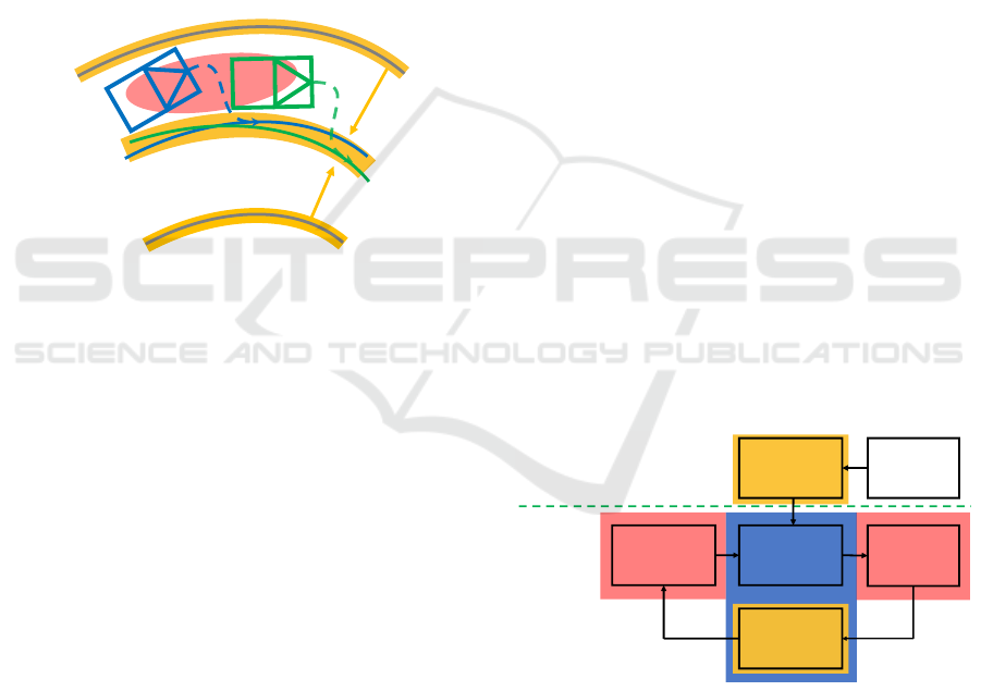
Figure 1: In the path-tracking problem, two types of uncer-

tainty can arise: 1) Localization uncertainty: Represented

by a red conﬁdence ellipse, this uncertainty leads to vari-

ations in the vehicle’s pose (position and orientation), de-

picted by dark blue and green lines. 2) Detection uncer-

tainty: Shown in yellow, this arises from inaccurate identi-

ﬁcation of lane boundaries, increasing uncertainty in calcu-

lating the reference path, illustrated by green and blue lines.

One remaining question is how the pure pursuit al-

gorithm performs under uncertainty, as illustrated in

Figure 1. This uncertainty can arise from GNSS inac-

curacies, resulting in various vehicle poses (positions

and orientations). Additionally, the accuracy of deter-

mining the reference path from road boundaries can

be inﬂuenced by the sensing capabilities of cameras.

To date, the study by (Kim et al., 2023) is the only

one that addresses pure pursuit under localization un-

certainty. In their approach, they established a 95-

percent conﬁdence interval around the reference path

and computed two possible steering angles based on

the boundaries of this interval. However, relying on

just two options may not be sufﬁcient to calculate the

optimal steering angle in the presence of uncertainty.

This work, therefore, proposes a method to derive

more representative steering angles. Given that lo-

calization noise is often assumed to follow a Gaus-

sian distribution, a more robust approach for deter-

mining them - known as sigma points - can be de-

rived using the unscented transform, a method typi-

cally applied in unscented Kalman ﬁlters (Wan and

Van Der Merwe, 2000). These sigma points are non-

linearly transformed based on the vehicle’s geometry

and reference path, and weighted to yield the optimal

steering angle.

Furthermore, the focus is on exploring pure pur-

suit algorithms under uncertainty for common road

types, such as straight and circular lanes (Kiencke

and Nielsen, 2000), with the goal of deriving closed-

form solutions for each road type - something that has

not been previously addressed for pure pursuit algo-

rithms. Clothoid lanes, which connect both straight

and curved lanes, are excluded from this work since

they can be simpliﬁed into circular cases. This re-

duction is done by ﬁrst deﬁning the waypoints us-

ing the method proposed by (V

azquez-M

endez and

Casal, 2016). A K-D tree is then used to identify the

waypoint closest to the vehicle, approximately corre-

sponding to the look-ahead distance. From this way-

point and its neighbors, the Menger curvature is cal-

culated, and its reciprocal gives the radius of the oscu-

lating circle. The process for circular lanes can then

be applied, as described in the subsequent section.

Additionally, it is assumed that the vehicle is

aware of the type of road it is on. The unscented trans-

form is employed to calculate a reasonably weighted

steering angle for the vehicle. The proposed algo-

rithm will be implemented in a Python environment

to assess its performance and compare its effective-

ness against the original pure pursuit algorithm under

uncertainty across different road geometries.

2.1: Generate

Sigma Points

2.3: Pure

Pursuit

Road

Model

2.4: Calculate

Weighted

Steering Angle

2.5: Update

Pose

Environment

Autonomous Vehicle

Unscented Transform

Kinematic Bicycle Model

Coordinate Transformation

2.2: Coordinate

Transformation

𝛿

𝓧

𝒊

𝓧

𝛿

𝑖

Figure 2: The general workﬂow of the proposed unscented

transform-based pure pursuit algorithm under uncertainty is

as follows.

2 METHOD

In Figure 2, the interaction between the two systems

- the environment and the autonomous vehicle - is il-

lustrated. The process begins with constructing the

Unscented Transform-Based Pure Pursuit Path-Tracking Algorithm Under Uncertainty

183

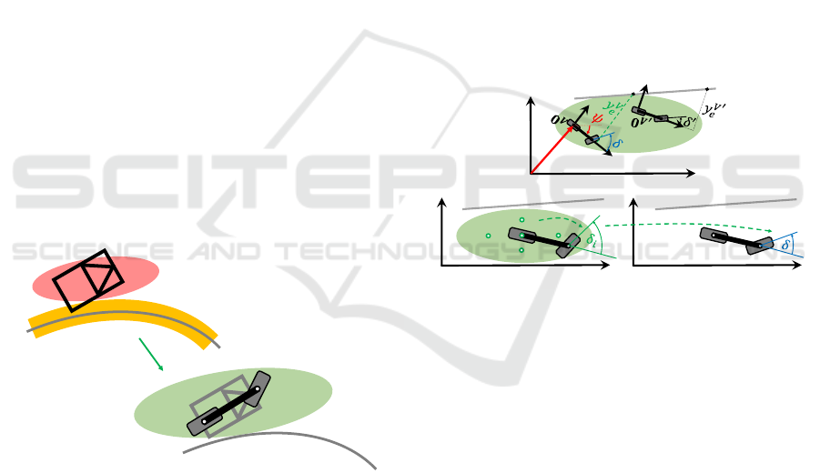
environment based on a road model, which consists

of straight or circular lines. The vehicle’s pose, de-

noted as X

X , is then deﬁned, and a set of sigma points,

, is generated, as described in Section 2.1. Subse-

quently, the road model is transformed from global

coordinates to the vehicle’s coordinate frame, as ex-

plained in Section 2.2.

These sigma points, along with the transformed

road, are then used to calculate the new steering an-

gles, δ

, using a pure pursuit algorithm based on the

kinematic bicycle model, as detailed in Section 2.3.

The weighted steering angle is then computed using

the unscented transform, outlined in Section 2.4. Fol-

lowing this, the vehicle’s pose is updated using the co-

ordinate transformation and the bicycle model (Sec-

tion 2.5), and the process of generating sigma points

is repeated.

In summary, Sections 2.1 and 2.4 incorporate the

unscented transform (highlighted in red), Sections 2.2

and 2.5 involve the use of coordinate transformations

(highlighted in orange), and Sections 2.3 and 2.5 ap-

ply the kinematic bicycle model.

2.1 Unscented Transform: Generate

Sigma Points

As depicted in Figure 1, there are two sources of un-

certainty in this problem: the vehicle’s localization

(V ) and the computation of the reference path (R).

𝜮

𝑽

𝜮

𝑹

𝜮

𝑽

∗

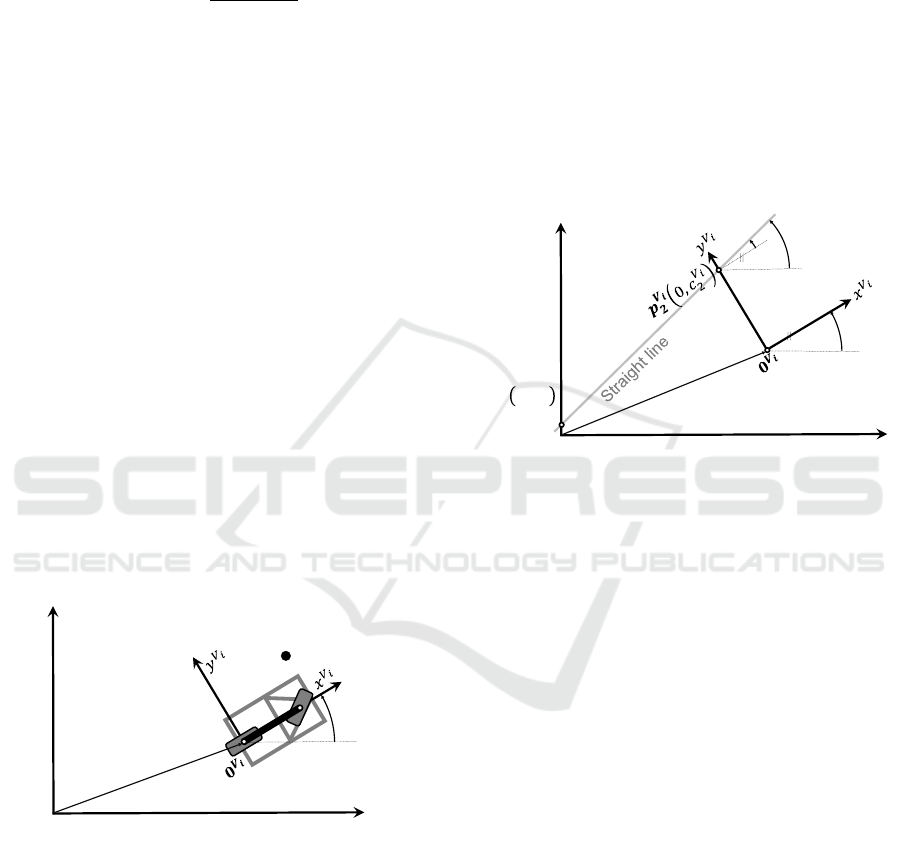
Figure 3: The calculation under uncertainty is simpliﬁed by

consolidating the various types of uncertainty—speciﬁcally,

the vehicle’s uncertainty (Σ

) and the road’s uncertainty

(Σ

) - into a single representation centered around the vehi-

cle, denoted as Σ

∗

As shown in Figure 3, the uncertainties are rep-

resented by their corresponding covariance matrices.

The covariance matrix for the vehicle’s localization is

given by:

= diag(σ

x,V

,σ

y,V

,σ

ψ,V

)

(1)

and is highlighted in red. Conversely, the covariance

matrix for the calculation of the reference path is rep-

resented as:

= diag(σ

x,R

,σ

y,R

,σ

ψ,R

(2)

which is highlighted in yellow. Note that diag denotes

a matrix with the provided values as its diagonal en-

tries, with zeros elsewhere. Additionally, σ

, σ

, and

represent the standard deviations of the vehicle in

the coordinates x, y, and ψ respectively, assuming in-

dependence between them.

As derived in (Zhu and Alonso-Mora, 2019), if

these uncertainties are independent, we can sum the

two covariance matrices, resulting in the total uncer-

tainty being attributed solely to the vehicle’s localiza-

tion. This resulting covariance matrix is represented

as:

∗

= diag(σ

,σ

)

= Σ

+Σ

(3)

which is illustrated in green. For computational sim-

pliﬁcation, the complex vehicle is replaced by the

kinematic bicycle model, as depicted in gray in Figure

𝑦

𝐺

𝑥

𝐺

𝟎

𝑮

𝓧

𝒊

𝑥

𝐺

𝑦

𝐺

𝟎

𝑮

𝒕

𝑦

𝐺

𝑥

𝐺

(𝑎)

(𝑏1)

(𝑏2)

𝟎

𝑮

𝒲

𝑖

𝑔

𝑖

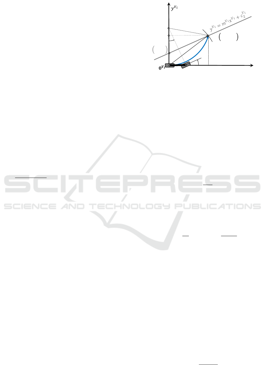
Figure 4: Tracking algorithm under uncertainty: (a) Differ-

ent poses result in different tracking errors, denoted as y

and y

′

, along with corresponding steering angles, δ and δ

′

(b) Unscented Transform: (b1) Different sigma points X

undergo a nonlinear transformation g

, resulting in steering

angles δ

. (b2) These angles are then weighted by W

produce the weighted steering angle δ.

With the incorporation of new uncertainty, the

pure pursuit algorithm is illustrated in Figure 4. The

vehicle’s coordinates are ﬁxed at its rear axle, denoted

by 0

), and undergo translation by t

t = [x

]

and rotation by ψ with respect to the global coordi-

nates 0

). Due to the uncertainty Σ

∗

, the ve-

hicle can assume multiple conﬁgurations, resulting in

multiple possible steering angles δ and δ

′

, as well as

cross-track errors y

and y

′

concerning the reference

path in gray, as depicted in 4 (a). Choosing all pos-

sible poses may be impractical. Therefore, according

to (Wan and Van Der Merwe, 2000), 2L

+ 1 sigma

points X

are selected from the distribution Σ

∗

, as

shown in Figure 4 (b1). Note that L

represents the

dimensionality of the pose, which is 3 in this case. Let

ICINCO 2024 - 21st International Conference on Informatics in Control, Automation and Robotics

184

X = [t

ψ]

represent the current pose, which serves

as the ”ﬁrst” sigma point:

= X

X .

(4)

The other 2L

= 6 sigma points are deﬁned as:

1...6

= X

+ λ

· ∆X

(5)

where ∆X

1,2

= ±[σ

,0,0]

, ∆X

3,4

= ±[0,σ

,0]

∆X

5,6

= ±[0,0,σ

]

, and L

as well as λ

are the

unscented parameters.

These inputs, namely X

and X

1...6

, will be uti-

lized in the coordinate transformation and unscented

transform steps, employing the bicycle model and

pure pursuit algorithm. Their propose is to calcu-

late the steering angles δ

, formulated as g

). Sub-

sequently, these steering angles will be weighted to

form the steering angle δ, as depicted in Figure 4 (b2).

2.2 Coordinate Transformation

Since roads are typically modeled in global coordi-

nates, while the pure pursuit algorithm uses the vehi-

cle’s coordinates to determine the reference point us-

ing the look-ahead distance, the concept of coordinate

transformation is introduced. This involves deriving

equations for converting points from global to vehicle

coordinates, and vice versa. These equations will then

be applied separately for straight and circular roads.

2.2.1 Points

𝑥

𝐺

𝑦

𝐺

𝜓

𝑖

𝟎

𝑮

𝒑

𝑮

↔ 𝒑

𝑽

𝒊

𝒕

𝒊

Figure 5: Transforming a point from the global coordinates,

denoted by p

, into the vehicle’s coordinates, denoted by

and vice versa.

In Figure 5, an autonomous vehicle is located at po-

sition t

= [x

t,i

]

and oriented at ψ

with respect

to the global coordinate system 0

. This pose can

correspond to one of the sigma points X

= [t

]

Let p

) and p

) represent a point p

p de-

scribed in the global and the i-th vehicle coordinates,

respectively. We can then transform p

to p

using

the following relationship:







cos(ψ

) − sin(ψ

)

sin(ψ

) cos(ψ

)







t,i



, (6)

or p

to p

using the following equation:







cos(ψ

) sin(ψ

)

−sin(ψ

) cos(ψ

)



− x

t,i

− y

t,i



. (7)

Utilizing these equations, we can represent the

roads and the sigma points in both coordinates, as will

be discussed in the subsequent sections.

2.2.2 Straight Lines









































 





 





Figure 6: Transforming a straight line from the global coor-

dinates into the vehicle’s coordinates and vice versa.

Given a straight line depicted in gray, as shown in Fig-

ure 6, it can be described in the global coordinate sys-

tem by:

= m

+ c

(8)

where m

denotes the slope of the straight line in the

global coordinates, while c

represents the y

inter-

cept, indicating where the line intersects the y

axis.

The subscript ”1” states that it is located at a speciﬁc

point, such as point p

Our task is to transform this straight line into the

i-th vehicle’s coordinate system described by:

= m

+ c

(9)

From Figure 6, it is evident that the intercept in the

coordinate, c

, corresponds to a different point,

denoted by p

, than point p

. The slope m

also

needs to be calculated. It is worth noting that all ideal

or noise-free waypoints must satisfy the line equation

(8).

In the global coordinates, it is evident that:

= arctan(m

(10)

where ψ

denotes the orientation of the straight line

from the x

axis. Upon further investigation into the

vehicle’s coordinates, the slope m

can be determined

Unscented Transform-Based Pure Pursuit Path-Tracking Algorithm Under Uncertainty

185

analogously using the angle ψ

and the yaw angle ψ

as:

= tan(ψ

) = tan(ψ

− ψ

(11)

By utilizing (7), we can transform the point

(0,c

) into the i-th vehicle’s coordinates p

as fol-

lows:







−x

cos(ψ

) + (c

− y

t,i

)sin(ψ

)

sin(ψ

) + (c

− y

t,i

)cos(ψ

)



(12)

Inserting this equation into the reformulated (9)

yields:

= y

− m

= x

t,i

(sin(ψ

) + m

cos(ψ

))

+(c

− y

t,i

)(cos(ψ

) − m

sin(ψ

)).

(13)

Using the sum formulas of sine,

sin(A + B) = sin(A) cos(B) + cos(A)sin(B),

(14)

and cosine,

cos(A + B) = cos(A) cos(B) − sin(A)sin(B),

(15)

results in:

cos(ψ

− ψ

)

t,i

sin(ψ

) + (c

− y

t,i

)cos(ψ

)).

(16)

Note that if the straight line is perpendicular to

the x

axis, this equation will not have a solution. In

other words, the y

intercept, denoted by c

, cannot

be determined.

2.2.3 Circles

Let a circle be described by its center point

) and has a radius of R

in the global co-

ordinates. Since the radius does not change, only the

center point is transformed using (7), resulting in:







cos(ψ

) sin(ψ

)

−sin(ψ

) cos(ψ

)



− x

t,i

− y

t,i



(17)

2.3 Pure Pursuit

The objective of this section is to determine the cross-

track error y

and the corresponding steering angle

for each sigma point X

. Employing the bicycle

model within the pure pursuit algorithm, the vehicle

is required to follow a circular path around the instan-

taneous center of rotation (ICR), located at the point

(0,R

) in the i-th vehicle’s coordinates, as depicted

in Figure 7 (Coulter, 1992). At the end, it reaches











 

























 



















 













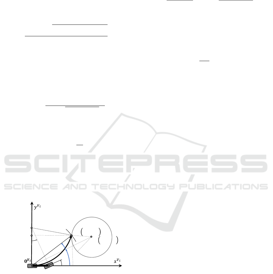
Figure 7: The look-ahead point D

in the vehicle’s coor-

dinates also lies along the straight line and is located at a

distance of d

from the rear axle.

the look-ahead point D

), determined by the

look-ahead distance d

from the rear axle, resulting in:

= (x

)

+ (y

)

(18)

By considering the triangle formed by points A,

, and ICR, we can establish the relationship:

= (x

)

+ (R

− y

)

= (x

)

+ (y

)

− 2R

+ R

(19)

Solving for R

yields:

(20)

Using the bicycle model, with the triangle formed

by the points ICR, 0

, and F

as shown in Figure 7,

we can derive the steering angle δ

using the radius

, the wheelbase L

and (20) as follows:

= arctan

. (21)

Typically, the adaptive look-ahead distance d

can

also be expressed as proportional to the current vehi-

cle speed v

with a proportionality constant K

, given

by:

= K

(22)

From (21), we only have to calculate the cross-

track error y

to ﬁnd the steering angle δ

. The deter-

mination of this error depends on the geometric type

of road, and its derivation will be done separately as

follows.

2.3.1 Straight Lines

Since (x

) lies on the straight line, as shown in

Figure 7, it must satisfy the reformulated (9):

− c

(23)

ICINCO 2024 - 21st International Conference on Informatics in Control, Automation and Robotics

186

In the case where m

= 0, we have the relation:

= c

(24)

otherwise, where m

̸= 0 inserting (23) in (18), solv-

ing the resulting quadratic equation and considering

that x

is positive, we obtain the formula for y

follows:

+ m

(1 + (m

)

− (c

)

1 + (m

)

(25)

2.3.2 Circles

To calculate the cross-track error y

, we require two

auxiliary angles α

1,i

, and α

2,i

, as can be seen in Fig-

ure 8. By examining the triangle 0

, D

, and C

and

applying the law of cosines, the ﬁrst angle α

1,i

is ob-

tained as follows:

1,i

= arccos

)

+ (y

)

+ d

− R

)

+ (y

)

(26)

There are two solutions for α

1,i

because cos(α

1,i

) =

cos(−α

1,i

). The angle α

2,i

is calculated as:

2,i

= arctan

. (27)

To maintain the vehicle’s current direction as

closely as possible, we need to use the smallest an-

gle, determined by α

min

← min|α

2,i

± α

1,i

As a result, this yields the cross-track error y

= d

sin(α

min

(28)























 



















 





















 



















Figure 8: Pure pursuit with a look-ahead point, D

, in the

circle’s circumference as a reference point for the vehicle.

2.4 Calculate Weighted Steering Angle

Let g

represent the nonlinear transformation of the

sigma point X

to the steering angle δ

= g

), as de-

picted in Figure 4 (b2). The resulting weighted steer-

ing angle δ can then be obtained as follows:

δ = W

+ W

1...6

∑

i=1

(29)

where the weights W

can be calculated according to

(Wan and Van Der Merwe, 2000):

+ λ

1...6

2(L

+ λ

)

(30)

2.5 Update Pose

After obtaining the steering angle δ, we rotate around

the instantaneous center of rotation ICR by the angle

β, using the bicycle model, where T denotes the up-

date time:

β =

tan(δ),

(31)

which results in the translation:

′

)

′

)

′

)



′

)

′

)



= v



cos(β)

sin(β)



, (32)

and in the orientation in the global coordinates:

′

= ψ + β.

(33)

Using Equation 7 yields the global position:

′

)

′

)

′

)



′

)

′

)





cos(ψ) − sin(ψ)

sin(ψ) cos(ψ)



′

)

′

)

′

)





(34)

Furthermore, the pose X

X = [t

ψ]

needs to be

updated by drawing from the normal distribution N

with the covariance Σ

∗

to account for uncertainties:

X ∼ N





′

)

′

)

′









0 0

0 σ

0 0 σ





. (35)

After the pose update, the procedure outlined in

Figure 2 is repeated.

3 SIMULATION

Now, the test scenarios for both straight and circular

roads are deﬁned, and the conventional pure pursuit

as well as the unscented transform pure pursuit algo-

rithms are qualitatively analyzed in the ideal case and

under uncertainty.

3.1 Setup

Implemented in Python, the straight road is deﬁned

as y

= 0, with m

= 0 and c

= 0, thus lying com-

pletely in the x

coordinate. Otherwise, the circular

road has a radius of R

= 5 m and a center point at

) = (0,R

). In both cases, the vehicle is set to

start at position t

t = [0 0.5]

m, oriented at ψ = 0

◦

The parameters for the unscented transform are

taken from (Wan and Van Der Merwe, 2000), with

Unscented Transform-Based Pure Pursuit Path-Tracking Algorithm Under Uncertainty

187

the dimensionality of the pose being L

= 3, α

0.001, and κ

= 0. The look-ahead gain is set to

= 1 s, similar to (Ohta et al., 2016). The vehi-

cle’s speed is v

= 1 m/s, and the vehicle’s length

is L

= 1 m. The standard deviations for the sum-

marized uncertainty are σ

= 0 m, σ

= 0.1 m, and

= 10

◦

. Note that the lateral distance from the ref-

erence path is also constrained to model the ﬁltering

capabilities, such as those of Kalman ﬁlter families, in

suppressing noise. The update time is set to T = 0.1 s.

Here, only a qualitative result analysis is conducted.

3.2 Results

Figure 9: Comparing the paths (x

) and the steering

angle δ using the unscented transform-based pure pursuit

(UTPP with uncertainty) and the pure pursuit (PP with

or without uncertainty) for straight roads (\wo stands for

”without noise”, and \w for ”with noise”).

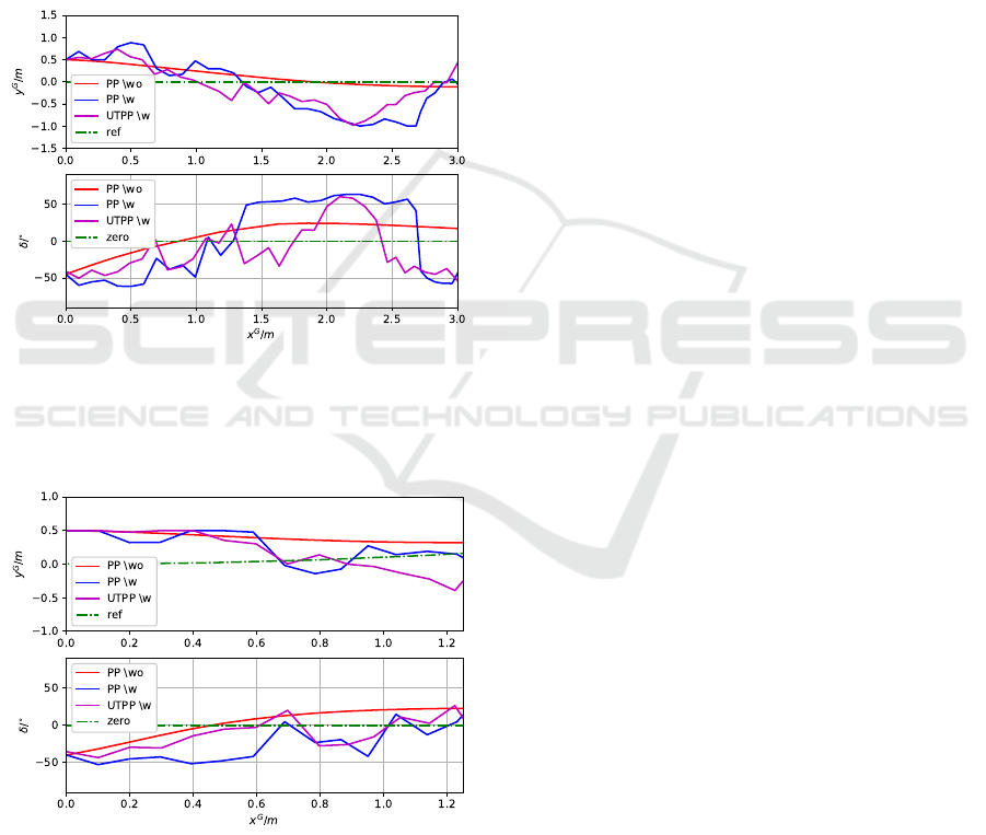
Figure 10: Comparing the results for circular roads, evaluat-

ing the paths (x

) and the corresponding steering angles

δ using the unscented transform-based pure pursuit (UTPP)

with uncertainty and the conventional pure pursuit (PP) with

and without uncertainty.

In Figures 9 and 10, the vehicle’s positions (x

)

over x

are illustrated. Under perfect sensing condi-

tions (denoted as wo), represented by the red tracks,

the vehicle effectively moves toward the reference

path shown in green, converging with oscillations

around it using the original pure pursuit (PP) algo-

rithm. This behavior results from the steering angle

δ calculated by the algorithm, where the vehicle ini-

tially steers right (indicated by a negative steering an-

gle) to stay aligned with the predeﬁned track, given its

initial position is to the left of the path. The steering

angle plot also oscillates around the zero angle, re-

ﬂecting the vehicle’s movement toward a straight tra-

jectory.

When noise is introduced (denoted as w), both the

conventional pure pursuit (PP) in blue and the un-

scented transform-based pure pursuit (UTPP) in ma-

genta demonstrate similar tendencies. Initially, both

algorithms steer the vehicle to the right to approach

the reference path, as indicated by the negative steer-

ing angles. However, the path generated by the un-

scented transform-based pure pursuit appears to con-

verge to the reference path more quickly than that of

the conventional pure pursuit under uncertainty. This

may be attributed to the use of multiple sigma points

(or steering angles) in the UTPP, which aids the ve-

hicle in returning to the track, as opposed to the con-

ventional pure pursuit, which relies solely on a single

calculated steering angle.

However, as the vehicle approaches the track, cer-

tain sigma points may cause it to deviate from the

path, as observed later in the simulation. Techniques

such as varying the look-ahead distance could help

mitigate this behavior, providing a potential avenue

for investigation in future studies.

4 CONCLUSIONS

An unscented transform-based pure pursuit algorithm

is proposed to address uncertainties in tracking ref-

erence paths across various road types. This method

effectively assists in guiding the vehicle back to the

track amidst noise. However, it may inadvertently

steer the vehicle away from the track once the ref-

erence path is reached. This behavior stems from the

algorithm’s current lack of adaptability in determin-

ing the look-ahead distance, which is an area of active

research.

Future improvements will focus on integrating

dynamically changing look-ahead distances to en-

hance the algorithm’s responsiveness. Additionally,

efforts will be made to develop the algorithm to au-

tonomously classify different road types. A gen-

eralized form of cross-track errors will be derived

to accommodate various road geometries, including

ICINCO 2024 - 21st International Conference on Informatics in Control, Automation and Robotics

188

clothoid roads. Furthermore, the integration of the

unscented Kalman ﬁlter for state observation will be

explored for more practical applications. Finally, a

quantitative analysis will be conducted to evaluate

the performance and limitations of the proposed ap-

proach.

REFERENCES

Cao, Y., Ni, K., Kawaguchi, T., and Hashimoto, S. (2024).

Path following for autonomous mobile robots with

deep reinforcement learning. Sensors, 24(2).

Chen, Y., Shan, Y., Chen, L., Huang, K., and Cao, D.

(2018). Optimization of pure pursuit controller based

on pid controller and low-pass ﬁlter. In 2018 21st In-

ternational Conference on Intelligent Transportation

Systems (ITSC), pages 3294–3299.

Coulter, R. C. (1992). Implementation of the pure pursuit

path tracking algorithm. Technical Report CMU-RI-

TR-92-01, Pittsburgh, PA.

Huang, Y., Tian, Z., Jiang, Q., and Xu, J. (2020). Path track-

ing based on improved pure pursuit model and pid. In

2020 IEEE 2nd International Conference on Civil Avi-

ation Safety and Information Technology (ICCASIT,

pages 359–364.

Joglekar, A., Sathe, S., Misurati, N., Srinivasan, S.,

Schmid, M. J., and Krovi, V. (2022). Deep rein-

forcement learning based adaptation of pure-pursuit

path-tracking control for skid-steered vehicles. IFAC-

PapersOnLine, 55(37):400–407. 2nd Modeling, Esti-

mation and Control Conference MECC 2022.

Kiencke, U. and Nielsen, L. (2000). Automotive Control

Systems: For Engine, Driveline and Vehicle . Springer-

Verlag, Berlin, Heidelberg, 1st edition.

Kim, K.-H., Na, H., Ahn, J., Shin, S., and Hwang, S.-H. H.

(2023). Modiﬁed pure pursuit algorithm robust to lo-

calization noise. In 36th International Electric Vehicle

Symposium and Exhibition (EVS36).

Kim, S., Lee, J., Han, K., and Choi, S. B. (2024). Vehi-

cle path tracking control using pure pursuit with mpc-

based look-ahead distance optimization. IEEE Trans-

actions on Vehicular Technology, 73(1):53–66.

Lee, J. and Yim, S. (2023). Comparative study of path track-

ing controllers on low friction roads for autonomous

vehicles. Machines, 11(3).

Li, B., Wang, Y., Ma, S., Bian, X., Li, H., Zhang, T., Li, X.,

and Zhang, Y. (2023). Adaptive pure pursuit: A real-

time path planner using tracking controllers to plan

safe and kinematically feasible paths. IEEE Transac-

tions on Intelligent Vehicles, 8(9):4155–4168.

Nan, J., Shang, B., Deng, W., Ren, B., and Liu, Y.

(2021). Mpc-based path tracking control with for-

ward compensation for autonomous driving. IFAC-

PapersOnLine, 54(10):443–448. 6th IFAC Confer-

ence on Engine Powertrain Control, Simulation and

Modeling E-COSM 2021.

Ohta, H., Akai, N., Takeuchi, E., Kato, S., and Edahiro,

M. (2016). Pure pursuit revisited: Field testing of au-

tonomous vehicles in urban areas. In 2016 IEEE 4th

International Conference on Cyber-Physical Systems,

Networks, and Applications (CPSNA), pages 7–12.

Qiang, F., Xiang, L., Xueyin, L., and Gonglei, L. (2021). An

improved pure pursuit algorithm for tractor automatic

navigation. In 2021 IEEE 4th International Confer-

ence on Information Systems and Computer Aided Ed-

ucation (ICISCAE), pages 201–205.

Rokonuzzaman, M., Mohajer, N., Nahavandi, S., and Mo-

hamed, S. (2021). Review and performance evaluation

of path tracking controllers of autonomous vehicles.

IET Intelligent Transport Systems, 15(5):646–670.

azquez-M

endez, M. E. and Casal, G. (2016). The

clothoid computation: A simple and efﬁcient numer-

ical algorithm. Journal of Surveying Engineering,

142(3):04016005.

Wan, E. and Van Der Merwe, R. (2000). The unscented

kalman ﬁlter for nonlinear estimation. In Proceedings

of the IEEE 2000 Adaptive Systems for Signal Pro-

cessing, Communications, and Control Symposium

(Cat. No.00EX373), pages 153–158.

Wang, R., Li, Y., Fan, J., Wang, T., and Chen, X. (2020).

A novel pure pursuit algorithm for autonomous vehi-

cles based on salp swarm algorithm and velocity con-

troller. IEEE Access, 8:166525–166540.

Wang, W.-J., Hsu, T.-M., and Wu, T.-S. (2017). The im-

proved pure pursuit algorithm for autonomous driving

advanced system. In 2017 IEEE 10th International

Workshop on Computational Intelligence and Appli-

cations (IWCIA), pages 33–38.

Wu, Y., Xie, Z., and Lu, Y. (2021). Steering wheel agv

path tracking control based on improved pure pur-

suit model. Journal of Physics: Conference Series,

2093(1):012005.

Yang, Y., Li, Y., Wen, X., Zhang, G., Ma, Q., Cheng, S., Qi,

J., Xu, L., and Chen, L. (2022). An optimal goal point

determination algorithm for automatic navigation of

agricultural machinery: Improving the tracking accu-

racy of the pure pursuit algorithm. Computers and

Electronics in Agriculture, 194:106760.

Zhao, S., Zhao, G., He, Y., Diao, Z., He, Z., Cui, Y., Jiang,

L., Shen, Y., and Cheng, C. (2024). Biomimetic adap-

tive pure pursuit control for robot path tracking in-

spired by natural motion constraints. Biomimetics,

9(1).

Zhu, H. and Alonso-Mora, J. (2019). Chance-constrained

collision avoidance for mavs in dynamic environ-

ments. IEEE Robotics and Automation Letters,

4(2):776–783.

Unscented Transform-Based Pure Pursuit Path-Tracking Algorithm Under Uncertainty

189