Research of Machine Learning and Feature Selection in Wine Quality

Prediction

Hongjun Zhang

Information Communication Technology, Xiamen University Malaysia, 43900 Sepang, Malaysia

Keywords: Wine Quality Prediction, Machine Learning, Deep Learning, Random Forest (RF), Feature Selection.

Abstract: As a globally renowned beverage, the competitiveness of wine in the market significantly hinges on its quality.

However, predicting wine quality proves to be a complex and intricate task due to its susceptibility to

numerous influencing factors. In this context, the present research endeavors to employ contemporary

machine learning methodologies to construct a dependable classification model aimed at accurately predicting

wine quality. This study juxtaposes the efficacy of four models, namely Support Vector Machine (SVM), K-

Nearest Neighbor (KNN), Random Forest (RF), and Artificial Neural Network (ANN). Furthermore, it

employs three feature selection techniques to exclude three features from the original eleven, thereby

enhancing model performance. Findings reveal that across this study, SVM consistently outperforms other

models, irrespective of the feature selection method employed. Additionally, it is noted that differing feature

selection methods exert discernible impacts on model performance. Assisting vintners and consumers in

accurately understanding and selecting high-quality wines, thereby fostering industry development and

enhancing consumer experiences.

1 INTRODUCTION

As a beverage with a long history, wine has a huge

market all over the world. The quality of wine will

greatly affect its sales, but wine identification is a

complex process. Because the quality of wine is

difficult to define because its structure is composed

of many aspects, there is a lack of a universally

recognized definition (Hoapfer et al., 2015).

Determining the quality of a wine based on individual

taste is a challenging task since everyone has their

own preferences and opinions on taste. However,

according to research, the quality of wine is affected

by many factors. Both the chemical components in

the grapes and the physical factors of the brewing

environment will determine the final quality of the

wine. A good wine is often particular about the

production process, including the careful selection

and planting of grapes, the fine control of grape

picking, fermentation, aging and other processes, as

well as the continuous innovation and optimization of

the brewing process. This process often requires a lot

of money and time. Wine quality used to be

determined by testing at the end of production, and if

the quality is not good, it would have to start from

scratch (Dahal et al., 2021). Therefore, accurate wine

quality prediction can optimize the production

process, reduce costs, thereby improving market

competitiveness and giving consumers a good

consumption experience. Therefore, a high-precision

model is of great significance in the prediction

process.

To predict wine quality, researchers have

considered numerous influencing factors and

developed various prediction methods. These

methods include prediction using active learning and

machine learning. There are currently multiple

datasets on wine quality, and each dataset contains

information on various chemical components of

wines of different qualities. Although the chemical

compositions collected vary, many researchers use

some modelling techniques on different datasets. For

example, Linear Regression (LR), RF, ANN, SVM,

and then analyse through the final model. Previous

studies have shown that the quality of the dataset has

a significant influence on the research findings since

it directly affects the model's capacity to explain and

predict. Hence choosing the best model becomes a

problem. The answer in the paper is to use dataset

preprocessing techniques and try to use different

models, and then give the best solution based on

specific research. The dataset used in this study is the

Zhang, H.

Research of Machine Learning and Feature Selection in Wine Quality Prediction.

DOI: 10.5220/0012982300004601

Paper published under CC license (CC BY-NC-ND 4.0)

In Proceedings of the 1st International Conference on Innovations in Applied Mathematics, Physics and Astronomy (IAMPA 2024), pages 5-12

ISBN: 978-989-758-722-1

WineQT Dataset from Kaggle. This is a real dataset

that collects the quality of Portuguese Vinho Verde

wines under various chemical factors. The target in

prediction is quality. The input feature is chemical

factors such as fixed acidity, residual sugar, pH,

alcohol, etc. This study will consider these

characteristics, build a prediction model, and

ultimately determine the optimal model by comparing

the quality of each model.

The present paper is structured as follows: In the

Section 2, the literature review will be used to

introduce the relevant work of the peer. In Section 3,

this paper discusses the proposed methods, including

the principles of the methods and the reasons for their

selection. In Section 4, this paper will examine the

experimental results, compare models, and select the

best model. In Section 5, the paper summarizes the

main findings and conclusions.

2 RELATED WORK

The quality of wine is affected by many factors,

including alcohol content, acidity, etc. Each

researcher chooses features differently to predict

wine quality. Natalie Harris et al. judge the quality of

wine through the aroma of wine (Harris et al., 2023).

Dragana B. Radosavljevic et al. judge the quality of

wine through the physical and chemical properties of

wine such as alcohol, ph, and density. The two

different methods each have their own advantages

(Radosavljevic et al., 2019). Considering more

factors in the research and selecting highly relevant

features can make it easier for researchers to predict

the quality of wine.

There have been many studies so far that have

explored various solutions related to wine quality

prediction, including machine learning and deep

learning. Among them, machine learning includes

Extreme Gradient Boosting (XGB), Adaptive

Boosting(AdaBoost), Gradient Boosting(GB), RF,

Decision Tree(DT), etc., and deep learning includes

ANN, Convolutional Neural Networks(CNN), etc.

Among them, Piyush Bhardwaj et al. used RF and

AdaBoost classifier to demonstrate their superiority

in predicting wine quality, and evaluated the model

from the aspects of Precision, Recall, F1, ROC_AUC,

and MCC (Bhardwaj et al., 2022). Feature selection

is an important factor that is frequently made during

model evaluation. RF, XGB, GB Classifier and Extra

trees classifier are used to select the top ten features

with Pearson correlation coefficient for training.

Keshab R. Dahal et al. conducted a comparative study

on the ensemble learning method Gradient Boosting

and the deep learning method ANN (Dahal et al.,

2021). In order to reduce the interference of the

dataset on the model, they used feature scaling

technology to reduce the scale difference between

features. Then, they evaluated the performance of the

model using three indicators: R, MSE and MAPE.

In addition to evaluating the performance of

different models on training datasets. Khushboo Jain

et al. evaluated the importance of data processing

techniques and feature selection for predicting wine

quality instead of focusing on various methods. In

machine learning and data mining, feature selection

is a research topic that has attracted much attention,

because different features have different effects on

the performance of the model. Agarwal et al.

considered the application of different feature

selection techniques such as principal component

analysis and recursive feature elimination in their

research. Piyush Bhardwaj et al. considered 54

features when predicting wine quality, and extracted

the 10 most important features through feature

selection. Six of these features were extremely

important in all models used in the experiment.

Current researchers mainly consider wine quality

prediction from three aspects. First, they focus on

datasets from different sources and predict wine

quality from various characteristics by collecting

datasets of different dimensions. Then consider

feature engineering, such as balancing the differences

between features through methods such as feature

scaling and identifying the most predictive features

through feature selection. Finally, they compare the

model's evaluation metrics and end up with a set of

models with the highest scores to determine the best

model.

3 METHODOLOGIES

In order to better understand the factors that affect

wine quality, this research will first conduct an

exploratory analysis of the data. Then the data is

preprocessed. After obtaining a suitable dataset, this

study will use this dataset to create and train different

models. These include KNN, RF, SVM, and ANN.

Finally, the final results will be obtained, and the

results discussed in depth. The flow chart is shown in

Figure 1.

IAMPA 2024 - International Conference on Innovations in Applied Mathematics, Physics and Astronomy

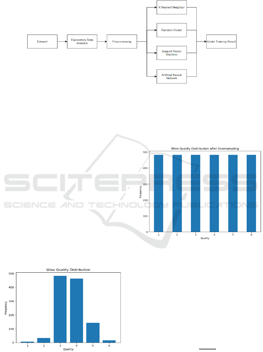
Figure 1: Research Workflow (Picture credit: Original).

3.1 Exploratory Data Analysis

In order to better analyse and understand the

distribution of data, this study uses exploratory data

analysis (EDA) to guide feature engineering in order

to understand the correlation between variables,

analyse data anomalies, etc., thereby providing

valuable suggestions for research. Detailed results

will be discussed in Section 4.

3.2 Preprocessing

Before establishing a wine quality prediction model,

the data set needs to be preprocessed. After analysing

the data set, it is found that there are no outliers and

missing values in the data set, so there is no need to

perform outlier processing and missing value

processing. By observing Figure 2, it can be

concluded that the distribution of wine quality is

unbalanced. There were significantly more samples

with quality grades "5" and "6" than samples with

other grades. Therefore, this research adopts

oversampling to balance the data set to improve the

model's performance on minority class samples.

Figure 2: Original Quality Distribution (Picture credit:

Original).

The results of oversampling are shown in Figure

3. In addition, considering the correlation between

features and prediction results, excluding low-

correlation features that have a small influence on the

dependent variable can help to obtain more accurate

prediction results (Gupta 2018).

Figure 3: Data Distribution after Oversampling (Picture

credit: Original).

In this dataset, there are significant differences

between different features, so an appropriate data

scaling method needs to be selected. According to

research results, the data scaling method will directly

affect the final evaluation index of the model (Ahsan

et al., 2021). Standardization and normalization are

both commonly used data scaling methods, and this

research uses standardization to make changes to the

dataset. After the features are standardized, the mean

becomes 0 and the standard deviation becomes 1. The

standardization formula is as follows:

𝑧=





(1)

Research of Machine Learning and Feature Selection in Wine Quality Prediction

In addition to data scaling, the data set is also

divided into a training set and a test set, of which the

training set accounts for 20%.

3.3 Model Selection and Construction

In this research, since the problem involved is a six

classification task, a broad classification model is

chosen to predict wine quality. These include the

ensemble learning model RF. and deep learning

models ANN. And trained two classic machine

learning models, KNN and SVM, as representatives

of traditional machine learning models. Each model

has its own advantages and limitations. This article

will comprehensively consider their performance and

applicability to better understand the effect of wine

quality prediction.

 K Nearest Neighbor

KNN is a non-parametric classification method, which

is simple but very effective in most cases (Guo et al.,

2004). The KNN algorithm calculates the distance

between the sample to be classified and the training

sample in the feature space, selects the k closest

training samples, and then votes or weights voting

based on the classes of these k training samples to

determine the class of the sample to be classified. In

this research, k=2. In KNN, the K is an important value,

which will directly affect the final result of the model.

If the K value is small, the generalization is poor, and

the model becomes complex and sensitive. If the K

value is large, the model will become simpler and

important features in the training set may be ignored.

The calculation formula of distance in KNN can be

expressed as:





∑



−x









(2)

Where different p corresponds to different distances.

This paper uses the Manhattan distance, p=1.

 Support Vector Machine

SVM is originally introduced as a binary classifier. It

has huge algorithmic advantages and is therefore

widely used in many fields. When SVM used as a

classification task, it is also called a support vector

classifier (SVC) and aims to find a hyperplane that best

fits the training data to maximize the margin and

minimize the prediction error.

SVM uses kernel techniques to extend linear

classification to nonlinear classification. Kernel

techniques can map input features into a higher-

dimensional space, making the data linearly separable

(Wang et al., 2008). Specifically, all the input features

xi of the wine and the true value yi of the

corresponding sample, which is the dependent

variable ‘quality’ of the wine, together form a training

set. The goal of SVM is to find a decision function

f(x) so that the model training result f(xi) can classify

samples into different classes as accurately as

possible. The basic form of SVM is shown in formula

(3).

𝑓

(

𝑥

)

=sign(

∑

𝛼



𝑦



𝐾(𝑥



,𝑥)+𝑏





) (3)

where x is the input feature vector, ai is the weight, K

(xi, x) is the kernel function, and b is the bias term.

 Random Forest

RF combines multiple decision trees into a more

powerful model. This method is also called ensemble

learning. RF adopts the Bagging method, which uses

bootstrap method to sample multiple times with

replacement from the original data, obtains a certain

number of bootstrap samples, and builds a decision tree

for all samples. RF is a classifier composed of many

decision trees, and its concept is similar to the "wisdom

of the crowd" (Radosavljevic et al., 2019). Each

decision tree can be regarded as a weak classifier, and

the RF combines the results of these weak classifiers

and derives the final prediction result. The merging

process is to vote or average the prediction results of

each decision tree. The decision formula, Dae et al.

uses formula 4 as shown.

𝐻(𝑥) =

∑

𝐼(ℎ



(𝑥)=𝑌)









(4)

Where x is the test sample data and hi is a single

decision tree. Y is the output variable, I is the indicator

function, and H is the combined result.

 Artificial Neural Network

ANN is a deep learning model established based on the

structure and operating principles of human neural

networks in biology (Tang 2022). A popular structure

in ANNs is Multilayer perceptron (MLP). ANN is a

classic deep learning model that consists of multiple

neurons arranged into multiple layers (input, hidden

and output layer). The neural network model

constructed in this study (Figure 4) consists of an input

layer, 3 hidden layers, and an output layer. Where the

output layer consists of 6 neurons, corresponding to the

6 qualities of wine.

IAMPA 2024 - International Conference on Innovations in Applied Mathematics, Physics and Astronomy

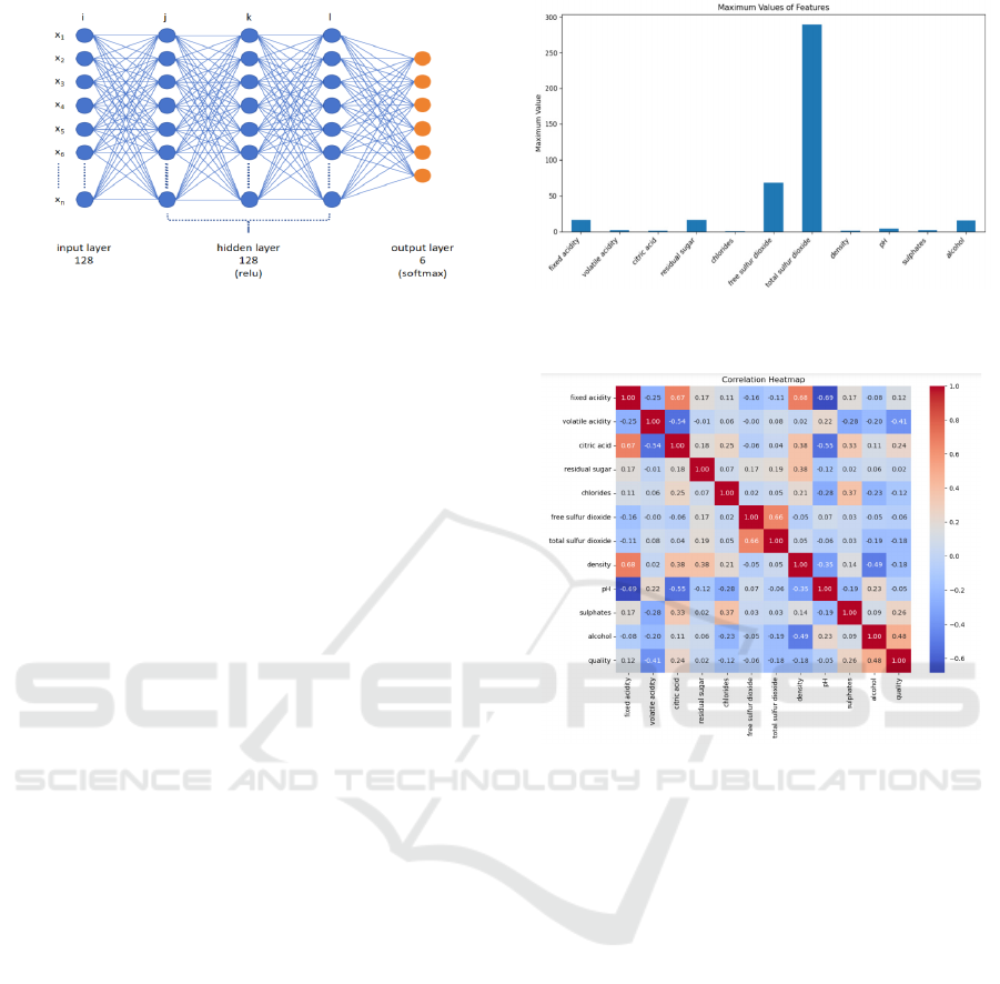
Figure 4: A Neural Network (Picture credit: Original).

Each neuron receives the input signal from the

neuron in the previous layer through a weighted

connection, and then applies an activation function to

obtain the output signal z (5).

𝑧=

∑

𝑤



𝑥



+𝑏





(5)

where w

is the weight, x

is the input signal, and b is

the bias term.

During the learning process, the neural network

will continuously adjusting the weight of the input

signal to learn, and adapt to different input data.

Ultimately, the neural network is able to classify or

predict the input data and generate corresponding

labels (Goodman and Zheng 2021).

4 EXPERIMENTAL SETUP AND

RESULTS

4.1 Dataset Overview

The dataset used in this paper contains 1599 wine

samples, but only 1143 wine samples are actually

seen because the void values have been filtered out.

The data type of all features is float. Each sample has

13 attributes (shown in Table 1).

Where Id is an irrelevant variable and therefore

does not participate in the discussion.

As mentioned in Figure 2 of Section 3, the data set in

this study is an unbalanced one. Therefore, it is

necessary to use methods to deal with imbalances to

make the quantity of quality consistent across different

labels. Figure 5 shows the distribution of the maximum

values of all features, which differ greatly in value. For

example, total sulfur dioxide compared to density.

Features with large numerical values may dominate the

model training process, resulting in a greater impact on

the model. Therefore, data scaling is used to ensure that

the model treats each feature fairly.

Figure 5: Maximum Values of Features (Picture credit:

Original).

Figure 6: Correlation Heatmap (Picture credit: Original).

As shown in Figure 6, this research uses heat map

to understand the release and changes of data, and

selects appropriate features for model training

according to the correlation among attributes.

According to the correlation matrix, since the

correlation between all features is less than 0.7, hence

there is no obvious collinearity between the features.

This shows that the correlation between the features is

moderate and will not have a great impact on the

model. In addition, when considering the label

"quality" used for prediction, it is observed that the

correlation of residual sugar, free sulfur dioxide, and

pH is less than 0.1. Therefore, in order to better train

the model, these features with too small correlation

coefficients are discarded in this paper. These

discarded features will not participate in model

training. The resulting training set size is (2318, 8) and

the test set size is (580,8).

Research of Machine Learning and Feature Selection in Wine Quality Prediction

Table 1: Description of Attributes in the Dataset.

Attribute Description

fixed acidity The amount of non-volatile acidic substances present in a fixed form

citric acid Acts as a preservative to increase acidity and enhance the taste of wine

residual sugar Sugars that are not fully converted to alcohol by yeast during brewing

chlorides The amount of salt in wine

free sulfur dioxide It is an additive used to protect the liquor from oxidation and microbial contamination

total sulfur dioxide Total amount of dimethyl sulfate and free sulfur dioxide

density The quality of wine per unit volume

pH Wine acidity level, usually between 3 and 4

sulphates An antioxidant and preservative that increases sulfur dioxide levels

alcohol It is the ethanol component made from the sugars in grapes that are fermented

quality The grade of the wine, the target to predict

Id Sample number

4.2 Experimental Settings

All models were implemented in the Python 3.12.0

environment. Hardware configuration includes

2.60GHz I7-9750,16GB RAM, and GTX1660T

All models are calibrated using grid search. The

specific Settings of the model are as follows.

 K Nearest Neighbor

The KNN model chooses Manhattan distance as a

distance metric, and considers the two nearest

neighbors for classification, and the nearest neighbor

has a higher weight.

 Support Vector Machine

The kernel of SVM is selected to be rbf. In the process

of model tuning, the hyperparameter gamma = 2 and

the penalty parameter C = 100 were selected.

 Random Forest

The maximum depth limit for each decision tree is 20,

the minimum number of samples on leaf nodes is 1, the

minimum number of samples required for node

splitting is 2, and 300 decision trees are included.

 Artificial Neural Network

The input layer, three hidden layers, and one output

layer make up the five layers of an ANN. The hidden

layer has 128 neurons. There are 128 neurons in the

three hidden layers, and the activation function is relu.

There are 6 neurons in the output layer, corresponding

to 6 kinds of wine quality, and the activation function

is softmax. The epoch of ANN is 50.

4.3 Evaluation Metrics

Accuracy, precision, recall, and F1 scores are the

metrics used to evaluate the model. These metrics are

used to evaluate the performance of the model.

 Accuracy

𝐴𝑐𝑐𝑢𝑟𝑎𝑐𝑦 =

   

   

(5)

It is the percentage of samples that the model correctly

identifies out of all samples. But it can be misleading

when the sample is imbalanced.

 Precision

𝑃𝑟𝑒𝑐𝑖𝑠𝑖𝑜𝑛 =

 

  

(6)

The number of samples true predicted as positive

divided by the total number of samples predicted as

positive by all models is known as precision.In multi-

classification, the precision of each class is weighted to

get the weighted-average precision.

 Recall

𝑅𝑒𝑐𝑎𝑙𝑙 =

 

  

(7)

Recall is the proportion of the model that successfully

predicts positive examples among all actual positive

examples.

 F1 Score

𝐹1=2 ∙

∙



(8)

The precision and recall weighted average is called F1.

F1 used to balance the prediction accuracy and

coverage of the model.

IAMPA 2024 - International Conference on Innovations in Applied Mathematics, Physics and Astronomy

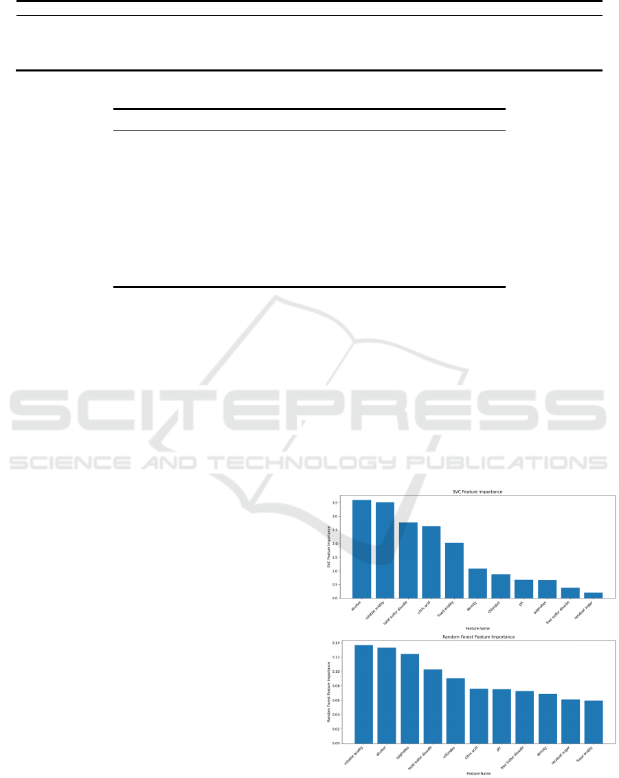
Table 2: Model Evaluation Results.

Model Accurac

Precision Recall F1 Score Time(s)

KNN 0.83 0.83 0.84 0.83 0.0049

SVM 0.85 0.85 0.85 0.85 0.33

RF 0.84 0.84 0.85 0.84 1.34

ANN 0.80 0.81 0.81 0.80 6.23

Table 3: Model Evaluation Results with SVM and RF Selection.

Feature Importance Model Accuracy Precision Recall F1 Score Time(s)

SVM

KNN 0.82 0.82 0.83 0.82 0.0039

SVM 0.82 0.82 0.83 0.83 0.33

RF 0.82 0.81 0.82 0.82 1.31

ANN 0.82 0.82 0.82 0.82 6.25

KNN 0.83 0.82 0.84 0.83 0.0040

SVM 0.84 0.85 0.84 0.84 0.35

RF 0.84 0.84 0.85 0.84 1.26

ANN 0.78 0.80 0.78 0.79 6.48

4.4 Model Evaluation

In order to evaluate the quality of wine, a total of four

models are used in this paper. The evaluation results

of these models are shown in Table 2.

In this research, all the models performed very

well. Their accuracy is maintained between 0.80 and

0.85. precision, recall and F1 are similar to the

accuracy and also maintain a high level. It shows that

the data preprocessing and model selection are done

well.

Furthermore, all four models performed similarly,

with accuracy above 0.80, but ANN performed the

worst. Although ANN is slightly less accurate than

the other models, its training time is significantly

higher, reaching 6.23s, almost five times that of RF.

This is expected, possibly because the amount of

training data is not enough to support its learning, so

the accuracy of the model is low. ANN is also a

complex model, so it takes a lot of time to train. As a

classical machine learning model, SVM performs

best. It not only achieved the highest accuracy of

0.85, precision of 0.85, recall of 0.85 and F1 of 0.85,

but also the training time is very short, only 0.33s. RF

is the same as SVM in recall, and other indicators are

also very similar, indicating that their performance is

similar. It is worth noting that KNN takes the least

time, only 0.0049s. Because its training process is

very simple, just save the training set. Then, when

making the prediction, KNN calculates the Manhattan

distance between the test sample and all the training

samples and votes to determine the classification of

the test sample based on the labels of the two nearest

neighbors in Manhattan. Nevertheless, KNN ended

up performing very well.

4.5 Feature Importance

In addition, two other feature selection methods are

used to further explore the effect of features on model

performance. The model is trained again by

discarding the three least important features selected

by SVM and RF respectively (Figure 7).

Figure 7: Feature Selection using SVM and RF (Picture

credit: Original).

Research of Machine Learning and Feature Selection in Wine Quality Prediction

In the feature selection method of SVM, the least

important features are sulphates, free sulfur dioxide

and residual sugar. In the feature selection method of

RF, the features that need to be discarded are density,

residual sugar and fixed acidity. Notably, residual

sugar is identified as a feature to be discarded in all

feature selection methods. It shows that residual sugar

may not be of great importance to the prediction of

wine quality.

In addition, under different feature selection

methods, the evaluation results of the model are

shown in Table 3.

The performance of KNN and RF remains basically

the same for the features extracted using RF, but they

both consume less time. SVM performance has

decreased slightly, accuracy, recall and F1 have all

decreased to 0.84, and training time has increased to

0.35s. In addition, ANN is significantly affected. The

ANN model performance decreases, the accuracy is

only 0.78, and the training time increases to 6.48s. This

feature selection is not a good method for SVM and

ANN, but it reduces the training time for KNN and RF

without affecting model performance. The

improvement may be more obvious in more large data

sets.

5 CONCLUSIONS

In summary, this paper used two learning methods,

machine learning and deep learning, respectively

trained four different classification models, and found

a suitable method to predict wine quality. These four

models are KNN, SVM, RF and ANN. Accuracy,

Precision, Recall and F1 Score are introduced as a

model of evaluation metrics. These models are

evaluated under 3 different feature selections. The

results show that each model exhibits different

performance under different feature selection

schemes. These different performances can provide

avenues for research on multiple aspects of the

model's impact on wine quality prediction. According

to the feature importance of SVM, the performance of

all models is similar. Features selected based on RF

decrease ANN performance. These two methods of

feature selection based on model results have a great

impact on ANN. In all cases, SVM performances the

best, predicting wine quality with the highest

accuracy. ANN slightly lagging behind the other

models. Although SVM shows better performance,

the advantages of ANN may be realized if the size of

the data set is increased. This paper mainly discusses

the prediction of wine quality by machine learning

and deep learning under different feature selection

schemes. In the future, larger data sets can be used,

and features can be studied from more aspects.

REFERENCES

H. Hoapfer, J. Nelson, S. E. Ebeler, H. Heymann ,

Molecules 20, 8453-8483 (2015)

K. Dahal, J.Dahal, H. Banjade, S. Gaire, OJS 11, 278-289

(2021)

N. Harris, C. Viejo, C. Barnes, A. Pang, S. Fuentes, Food

Biosci. 56, 1-16 (2023)

D. Radosavljevic, S. Ilic, S. N. Pitulić, A Data Mining

Approach to Wine Quality Prediction , in

Proceedings of International Scientific Conference, 1-6

(2019)

P. Bhardwaj, P. Tiwari, K. Olejar, W. Parr, D. Kulasiri,

MLWA, 8, 1-11 (2022)

K. Jain, K. Kaushik, S. K. Gupta, S. Mahajan, S. Kadry, Sci

Rep 13, 1-18 (2023)

G. Agrawal, D. K. Kang, Int. J. Internet Broadcast.

Commun. 10, 25–30 (2018)

Y. Gupta, Procedia Comput. Sci 125, 305-312 (2018)

M. Ahsan, M. Parvez Mahmud, P. K. Saha, K. D. Gupta, Z.

Siddique, Technologies 9, 52 (2021).

G. Guo, H. Wang, D. Bell, Y. Bi, K. Greer, KNN Model-

Based Approach in Classification. in Proceedings of

The Move to Meaningful Internet Systems 2003:

CoopIS, DOA, and ODBASE, OTM, 986-996

(2004)

G. Wang, D. Y. Yeung, F. H Lochovsky, IEEE T. Neural

Networ. 19, 1753-1767 (2008)

R. N. Behera, K. Das, IJIRCCE 5, 1301-1309 (2007)

D. Tang, Adv. Appl. Math 11, 3053-3059 (2022)

R. M. Goodman,Z. Zheng, A learning algorithm for multi-

layer perceptrons with hard-limiting threshold

units, Workshop on Neural Networks for Signal

Processing, 219-228 (2021)

IAMPA 2024 - International Conference on Innovations in Applied Mathematics, Physics and Astronomy