Ensemble Learning Based Models for Planet Classification

Xiyue Wang

School of Mathematics, Jilin University, Changchun, 130000, China

Keywords: Machine Learning, Ensemble Learning, Classify Planets, Neural Network.

Abstract: Astronomers explore various phenomena and laws in the universe through observation, experimentation, and

theoretical models to gain a deeper understanding of the structure, composition, and evolution of the universe.

There are many unanswered questions in astronomy, such as how to properly classify planets. At the same

time, appropriate classification methods can deepen people's understanding of astronomy. In the past, many

scholars have speculated on classification criteria. The purpose of this study is to explore a satisfactory model

for planet classification and provide a reliable reference for subsequent researchers. Furthermore, this article

utilizes a variety of machine learning methods and deep learning models, including Linear Regression,

Principal Component Analysis, Linear Support Vector Machine, Random Forest, XGBoost Regression and

Artificial Neural Network. Among all models, ensemble learning methods Random Forest and XGBoost

produce the best results, the former of which achieved an adjusted of 0.96 and XGBoost obtained an adjusted

of 0.95. In addition, we make estimates for future research and provide improvements.

1 INTRODUCTION

In 2006, the IAU Association defined what are

planets in the solar system. However, planets outside

solar system are still not clearly defined. Therefore, it

is essential to define systematically what a planet is.

In general, planets have many physical properties,

such as temperature, humidity, luminosity, radius,

size, etc. Obtaining a relatively complete planetary

physical model is very important for astronomy,

which is equivalent to laying the foundation for

subsequent research. Because of that, a suitable

model for determining planets is needed.

In order to arrive at a suitable and complete

definition of a planet, many efforts have been made

to consider the various factors that influence it. Many

researchers have applied model building methods

such as cluster analysis, factor analysis, decision

trees, and random forests on different data sets and

analyzed different situations.

In line with previous research, we found fact that

the quality of the dataset significantly affects the

results of study. The dataset we utilized in this study

is the planet classification prediction set from Kaggle,

which is a dataset containing 240 stars in 6 categories.

The target feature in the prediction is classification

using the shape of stars in celestial space. The

independent variables, such as temperature, radius,

absolute shock, color, spectral level and etc. are also

taken into consideration.

Some related research reports on Kaggle

conducted to finish high-precision training and

prediction on the same data set. It shows high quality

from data preprocessing to split training sets and test

sets. In addition, it is very important to choose the

most appropriate method during the research process,

and various factors need to be considered to

determine the model.

To select some relatively suitable models, this

study attempts various types of models and makes

judgments based on the results obtained. We studied

this star dataset from many aspects. At the same time,

it is compared with many advanced machine learning

models, thereby achieving an efficient integrated

learning method.

The main difference between this research and

previous researches is that we studied this Star dataset

from many aspects and angles. At the same time,

comparing with many advanced machine learning

models, we implemented an efficient integrated

learning method and further compared and judged

better classification models. For example, for deep

learning, we use convolutional neural network

(CNN); for integrated learning, we utilize random

forests and XGBoost; for traditional machine learning

Wang, X.

Ensemble Learning Based Models for Planet Classiﬁcation.

DOI: 10.5220/0012992000004601

Paper published under CC license (CC BY-NC-ND 4.0)

In Proceedings of the 1st International Conference on Innovations in Applied Mathematics, Physics and Astronomy (IAMPA 2024), pages 60-67

ISBN: 978-989-758-722-1

methods, we also use linear regression and PCA as

benchmark models to complete the comparison.

There are the frame of this paper: We finished

introducing related work by showing each category of

prediction stars’ types in Section 2. We describe the

details of our methods in Section 3, including our

reasons for choosing these methods and the theories

of methods are introduced. After that, we examine the

experimental results and analyze them in Section 4.

Last but not least, the conclusion of this study is listed

in Section 5 with references showing at the end.

2 RELATED WORK

In the beginning, some scientists used a single

parameter to classify stars. At first, Michael and

Meghar classified the differences in quality, and

classified different orders of magnitude into one

category, which is a very traditional way (Swedenborg

1973 & See 1909). Then Fischer and others classified

stars with different densities by taking into account

differences in composition, but it was still not perfect

(Fischer et al., 2014). After that, Chen and Kipping

analyzed the mass-radius relationship of planets and

then classified them (Chen and Kipping, 2017).

Furthermore, Marley and others proposed a

classification method based on components through

the study of spectra. But none of these methods have

very good results (Marley et al., 1999).

However, the method of classifying a single

variable is not more accurate than considering many

variables at the same time. Therefore, many

subsequent scientists will consider many variables at

the same time in the problem of star classification.

Furthermore, there are many factors that need to

be considered when predicting star type. At the same

time, the more factors we consider, the easier it is for

us to conduct research. First of all, Stern and

Levinson proposed a classification method based on

quality and composition in 2002. On the other hand,

they showed that such classification methods are

imperfect and proposed seven requirements that

should be met to build a classification framework.

After that, the classification method introduced by

Russell in the article took into account the three

properties of the planet's composition, mass, and

orbit. The mutual combination of the three aspects

constitutes the final classification. Later, in

FANDOM's introduction to planet classification, the

classification framework took into account the

planet's mass, orbit, surface state, and composition.

They are also various solutions having been used

for planet type classification and prediction in the

past, including machine learning methods and deep

learning models.

First of all, Dieleman and others trained

convolutional neural networks on galaxy images and

established a model to achieve fine-grained galaxy

morphology classification with very high accuracy

(Dieleman et al., 2015). Secondly, Huertas-Company

and others used deep convolutional neural networks to

classify the morphological catalog of 50,000 galaxies

in the H-band (Huertas-Company, 2015). Kim and

Brunner trained a deep CNN to establish some image

classification models for star-galaxy (Kim and

Brunner, 2017). Then Dom´ınguez S´anchez and

others used convolutional neural networks to provide

two classification methods: Hubble sequence T-type

and Galaxy Zoo 2 morphological classification

methods (Dom´ınguez S´anchez et al., 2018). After

that, Lukic and Br¨uggen also applied deep neural

networks to train classification models on data sets

(Lukic, 2017). Moreover, Aniyan and Thorat used a

convolutional neural network improved other model

for morphological classification (Aniyan and Thorat,

2017).

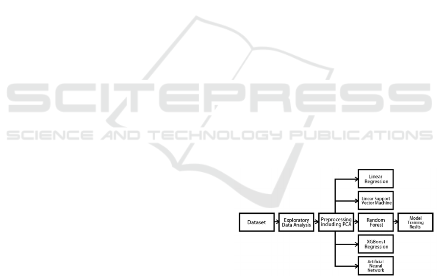
In this research, we first conduct exploratory data

analysis on the dataset and preprocess the input data.

Then we construct and train several machine learning

models, including Linear Regression (LR), Principal

Component Analysis (PCA), Linear Support Vector

Machine (SVM), Random Forest (RF), XGBoost

Regression (XGB) and Artificial Neural Network

(ANN) to obtain corresponding results for further

analysis. Figure 1 shows the workflow of our study in

this paper.

Figure 1: Research Workflow (Picture credit: Original).

3 METHOD

3.1 Exploratory Data Analysis

In the first part, about conducting exploratory data

analysis, the aim is to provide valuable insights about

the data set. The analysis covers data distributions,

Ensemble Learning Based Models for Planet Classiﬁcation

feature connotations, variable correlations, etc.

Detailed results are provided in Section 4.

Before establishing and training a planet

classification model, data preprocessing is required to

ensure the accuracy of the answer. Since the dataset

used has been processed by Stefan-Boltzmann's law

of Black body radiation, Wienn's Displacement law,

Absolute magnitude relation and Radius of a star

using parallax, there are no missing values now. And

because of that, there is no need to consider this

aspect.

However, there are some qualitative values about

the planet class in the dataset, which should be

specially consider. And also taking into account the

correlation with the predicted label, some features

whose correlation coefficient is not high enough will

be discarded and no longer considered. In addition to

it, the original dataset is split into a training set and a

test set.

3.2 Model Selection and Construction

In this study, we choose to implement five kinds

integrated learning models to classify planets. In

addition, Integrated Learning has the advantage of

combining multiple machine learning algorithms.

Therefore, the learning models obtain by this method

can achieve better prediction performance than using

any other component algorithm alone.

Integrated Learning consists of many of its base

learners, which are usually created from basic

learning algorithms such as Decision Trees and

Neural Networks.

For this study, for ensemble learning, we choose

to utilize SVM, RF and XGB; for deep learning, we

use CNN; and for more traditional machine learning

methods, we also use LR and PCA as benchmark

models for comparison.

 LR

The goal of linear regression is to fit a linear model

with the smallest RSS between the true values and

predicted values.

𝑌



=𝛽



+𝛽



𝑋



+𝛽



𝑋



+⋯+𝛽



𝑋



+𝜀



, 𝑖 = 1, ⋯ , 𝑛 (1)

In the historical process of scientists studying star

classification, they discussed linear regression at first,

that is, the influence of an independent variable.

Nowadays, there are multiple factors have to be

considered, and it can be expressed in the matrix

form.

 PCA

Another classical modeling method, Principal

Component Analysis (PCA), with hoping to obtain

the items with the largest impact as the main criteria

for judging planets. It is using orthogonal

transformation to linearly transform a series of

observations of possibly related variables. In this

dataset, it is equivalent to exploring the proportion of

each independent variable.

 SVM

SVM is an ensemble learning model, whose purpose

is to solve complex classification problems, etc.

𝝎



⃗

⋅𝒙



⃗

−𝒃=𝟎 (2)

As an extension of the perceptron, on the one

hand, SVM can minimize the empirical error; on the

other hand, it can make the area the largest at the same

time.

 RF

RF is an advanced ensemble learning model. It is

equivalent to an advanced version of the decision

trees. The RF algorithm always introduces additional

randomness by searching for the maximum attribute

in a random subset of features during node splitting.

On the other hand, when making predictions for

regression tasks, RF takes the average of all single

decision tree estimates.

In this study, all trees in the forest are averaged to

obtain the final result.

 XGB

XGB is a malleable decentralized GBDT machine

learning system. Just like random forest mentioned

earlier, gradient boosting is also one of the Bagging

extension.

The GBDT model trains an ensemble of decision

trees in an iterative manner. In every iteration, they

all use the previously obtained residuals for fitting,

and the final answer is the weighted sum of all

predictions. Therefore, it is equivalent to an improved

random forest method.

XGB was born to enhance the performance of

machine learning models and increase computing

speed. It is a highly accurate and scalable

implementation of GBDT that has gained great

popularity.

 ANN

The Artificial Neural Network (ANN) is a neural

network model, which uses mathematical operations

called convolutions in at least one layer instead of

general matrix multiplication.

A neural network has multiple layers of neurons.

Deep neural networks typically have one input layer,

one output layer and some hidden layers. As an

IAMPA 2024 - International Conference on Innovations in Applied Mathematics, Physics and Astronomy

example, a 2-hidden-layer deep neural network is

depicted in table 1.

Table 1: ANN network.

ut La

Hidden La

er 1 110 neurons

Hidden Layer 2 60 neurons

Out

ut La

1 neuron

This is done by each neuron receiving input

signals from the previous layer of neurons through

weighted connections, comparing the weighted sum

of the received signals with the threshold, and in turn

training the network by adjusting the weights.

4 EVALUATION RESULTS

4.1 Experimental Setting

In this study, we employed several hyperparameters

to optimize the performance of our machine learning

models. Notably, we used Cost Complexity Pruning

Alpha values to manage the complexity of our

decision trees, and a minimum impurity decrease

value set at 0.0. Additionally, we set the minimum

samples per leaf and the minimum samples required

to split a node to 1 and 2, respectively. The optimal

‘ splitter ’ parameter was carefully selected to

enhance model performance.

Evaluation Metrics:

The models were evaluated using multiple metrics

to ensure comprehensive model assessment.

Specifically, the metrics used were Mean Absolute

Percentage Error (MAPE), Root Mean Squared Error

(RMSE), Root Mean Squared Logarithmic Error

(RMSLE), and Adjusted R².

MAPE: This metric provides a percentage error

and is easier to interpret. The smaller the MAPE

value, the better the prediction effect.

RMSE: RMSE measures the square root of the

average of squared differences between prediction

and actual observations. It is more sensitive to outliers

because the effect of each error is squared.

RMSLE: As a variant of RMSE, RMSLE applies

a logarithmic scale to both predicted and actual

values. This makes it robust against larger errors and

works well when there are exponential growth

patterns in the data.

Adjusted R²: This metric adjusts the Coefficient

of Determination by accounting for the number of

predictors in the model. Adjusted R² increases when

a useful variable is added to the model and decreases

when a non-useful variable is added, thus helping in

determining the goodness of fit while penalizing for

unnecessary predictors.

4.2 Dataset Overview

This paper utilizes the Star dataset to predict star

types from Kaggle. It had been took by Sloan Digital

Sky Survey and comprises data about 100,000 results

in space. Each entry in the dataset consists of 17

feature columns and 1 category information column.

The stars in the dataset are divided into three

categories: GALAXY, STAR, and QSO. The

comparison of their numbers is shown in Figure 2.

GALAXY has 55,561, while QSO has only 12,133.

There is a big difference between the two numbers.

Figure 2: Type classification (Photo/Picture credit: Original).

Ensemble Learning Based Models for Planet Classiﬁcation

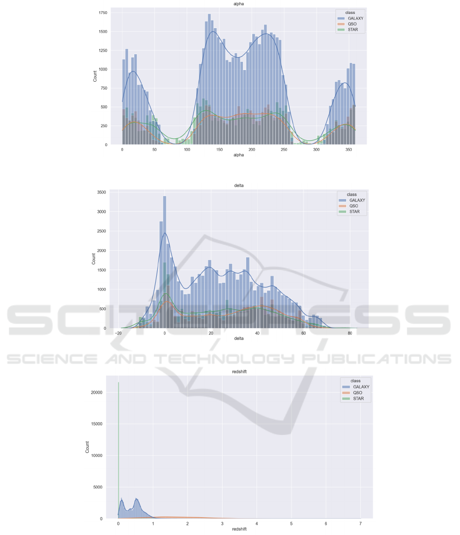
Figure 3: About Alpha Correlation (Picture credit: Original).

Figure 4: About Delta Correlation (Picture credit: Original).

Figure 5: About Redshift Correlation (Picture credit: Original).

IAMPA 2024 - International Conference on Innovations in Applied Mathematics, Physics and Astronomy

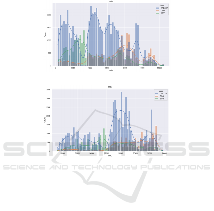
Figure 6: About Plate Correlation (Picture credit: Original).

Figure 7: About MJD Correlation (Photo/Picture credit: Original).

4.3 Feature Importance Exploration

Classifying according to different features, some

results were obtained, among which the results for

astronomical numbers (such as alpha, u, redshift, etc.)

were relatively good. It is also necessary to use

logarithmic form to better present the results when

they are not clear.

What follows is a series of images exploring what

factors are relatively large for classification (Figure 3,

figure 4, figure 5 figure 6 and figure 7). The blue line,

orange line and green line are the fitting lines for

GALAXY, QSO and STAR respectively.

We also deeply explored the correlations between

all attributes, hoping to have a more appropriate

comprehension of the data. At the same time, the

"redshift" variable get the highest correlation with

"class" and the "u" variable with the second highest

correlation were found (Figure 8).

4.4 Model Evaluation

These 5 models are evaluated using the evaluation

metrics mentioned in 3.4. The answers obtained are

displayed in table 2.

Among all the models, as expected due to the

characteristics of the data set, the linear regression

model performed the worst, very poorly.

For RMSE, LR has the highest results and ANN

has the lowest. And for RMSLE, every result except

LR is similar in size. Then, for MAPE, ANN obtained

smaller results.

As representatives of integrated learning methods,

Random Forest and XGBoost produced equally

satisfactory results and outperformed other models

for all mentioned metrics.

Ensemble Learning Based Models for Planet Classiﬁcation

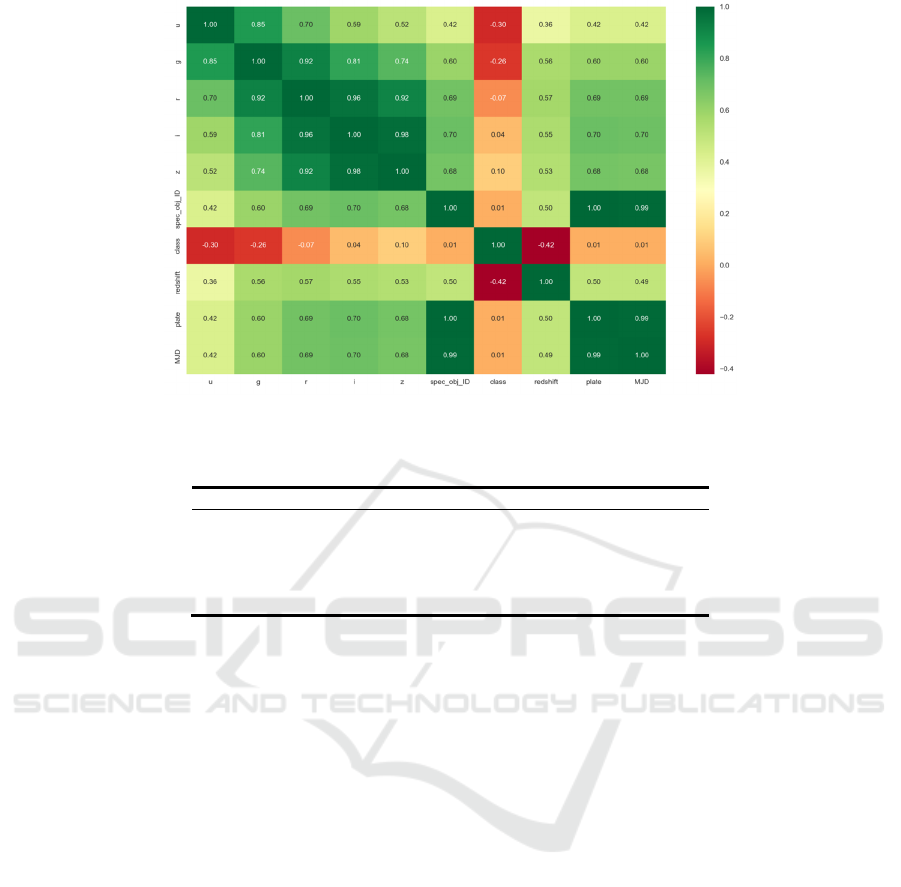
Figure 8: Correlation (Photo/Picture credit: Original).

Table 2: The evaluation result.

Model Accurac

RMSE RMSLE MAPE R²

LR 0.23 0.93 0.59 2.98212×10^{15} 0.20

SVM 0.90 0.36 0.23 4.19876×10^

{

}

0.82

RF 0.97 0.17 0.12 7.38897×10^{15} 0.96

XGB 0.97 0.19 0.13 9.29750×10^

{

}

0.95

ANN 0.73 0.05 0.1415 0.10 0.93

However, for SVM’s performance, the results are

in the middle position, not reaching the level of

as 0.9 like that of RF and XGB, but it also achieved

good results (0.83).

Furthermore, ANN also makes good predictions,

on the other hand it is the most time-consuming all of

them. Among them, random forest has the best result.

5 CONCLUSION

In summary, this paper includes both machine

learning and deep learning to find a suitable method

to better classify planets. At the beginning of it, the

current state of the planetary classification industries

is described. Then some visualizations are given in

the article, explaining the steps more clearly, such as

the correlation between factors. After that, some

models are given, which used are Linear Regression,

SVR, XGBoost, Random Forest and Neural Network.

Among all of these models, two ensemble learning

methods, Random Forest and XGBoost do the best

job. Specifically about that, we use 100 trees to build

a random forest. Subsequently, the mean square error

is used as the segmentation criterion. Therefore,

satisfactory results are obtained: the RMSE is 0.17,

RMSLE is 0.12, MAPE is 7.38897×10^{15}, and the

adjusted

is 0.96. with 0.19 in RMSE, 0.13 in

RMSLE, 9.29750×10^{15} in MAPE and 0.95 in

, and it has an accuracy of 0.85 and RF is 0.91. In

future experiments, we hope to obtain better results

for classifying planets. There are ways to enhance the

number of fitting experiments and bring up the

accuracy of answers to get a more accurate

classification method.

There are some ways to increase the number of

fittings and improve the accuracy of the answers to

get a better classification method.

REFERENCES

Swedenborg E. Latin: Opera Philosophica et Mineralia

(English: Philosophical and Mineralogical Works).

Principia, 1973: 1

See T J J. Proceedings of the American Philosophical

Society, 1909, 48(191): 119

Fischer D A, Howard A W, Laughlin G P, et al. In: Beuther

H, Klessen R S, Dullemond C P, et al, eds. Protostars

and Planets VI. Tucson: University of Arizona Press,

2014: 715

Chen J, Kipping D. Physics and Chemistry of the Earth,

2017, 834(1): 17

IAMPA 2024 - International Conference on Innovations in Applied Mathematics, Physics and Astronomy

Marley M S, Gelino C, Stephens D, et al. Physics and

Chemistry of the Earth, 24, 5, 1999, 573-578

Dieleman S, Willett K W, Dambre J. Monthly notices of the

royal astronomical society, 2015, 450: 1441

Huertas-Company, Gravet R, Cabrera-Vives G, et al.

Physics and Chemistry of the Earth, 2015, 221(1): 8

Kim EJ, Brunner R J. Monthly notices of the royal

astronomical society, 2017, 464: 4463

Dom´ ınguez S´anchez H, Huertas-Company M, Bernardi

M, et al. Monthly notices of the royal astronomical

society, 2018, 476: 3661

Lukic V, Br¨uggen M. IAU Symposium, 2017, 325: 25

Aniyan A K, Thorat K. Physics and Chemistry of the Earth,

2017, 230(2): 20

Ensemble Learning Based Models for Planet Classiﬁcation