Implementation of 12 Transition Controls for Rotary Double Inverted
Pendulum Using Direct Collocation
Doyoon Ju
a
, Taegun Lee
b
and Young Sam Lee
c
Department of Electrical and Computer Engineering, Inha University, Incheon, Korea
Keywords:
Rotary Double Inverted Pendulum, Transition Control, Direct Collocation, Optimal Control.
Abstract:
The rotary double inverted pendulum system has one stable and three unstable equilibrium points due to
its kinematic properties. This paper extends the traditional swing-up control problem by defining a novel
transition control problem among these points. We formulate the system’s dynamic equations and boundary
conditions for different equilibrium points to minimize energy consumption during transitions, resulting in a
two-point boundary value optimal control problem. This problem is solved offline to calculate the feedforward
trajectory for feedforward control. To convert the continuous optimal control problem with constraints into a
nonlinear optimization problem, we employ the direct collocation method. A time-varying Linear Quadratic
controller is used as the feedback controller to accurately track the generated feedforward path during real-time
control, compensating for uncertainties. Previous studies on rotary double inverted pendulums have focused on
the swing-up problem, with no research addressing transition control between the four equilibrium points. This
paper defines the transition control problem for the rotary double inverted pendulum and proposes a control
strategy. The method’s effectiveness and practicality were validated through the design and implementation
of 12 transition trajectories in experimental settings, successfully demonstrating its feasibility and utility.
1 INTRODUCTION
The inverted pendulum system, with its unstable dy-
namic characteristics, incorporates both nonlinear and
non-minimum phase properties, making it a widely
used educational tool for teaching control theory.
Additionally, it serves as a popular testbed for re-
searchers to validate new control techniques. Ma-
jor studies on the inverted pendulum system include
swing-up control, which transitions the pendulum
from an initial state where it points downward to an
upright state(
¨
Astr
¨
om and Furuta, 2000; Meta et al.,
2014), and balance control, which aims to maintain
stability in the upright state after the swing-up(Oh and
Lee, 2018). Among these, swing-up control is consid-
ered a more challenging research topic compared to
balance control because it requires designing a con-
troller that accounts for the system’s nonlinearity, in-
stability, and input/output constraints.
In the case of the rotary inverted pendulum sys-
tem, unlike the linear inverted pendulum where the
a
https://orcid.org/0000-0001-7011-6779
b
https://orcid.org/0009-0007-3107-2735
c
https://orcid.org/0000-0003-0665-1464
pendulum is fixed to rotate in a single plane, the
powered arm of the rotary inverted pendulum also
rotates. This characteristic allows the pendulum to
move within a three-dimensional space, introducing
additional challenges in performing swing-up control.
To address the swing-up problem of such a rotary in-
verted pendulum system, various methods have been
applied, including self-tuning techniques(Ratiroch-
Anant et al., 2004), PID controllers(Rahairi et al.,
2011), and methods utilizing sliding observers(Thein
and Misawa, 1995). Recently, research has also
been conducted to solve this problem using artifi-
cial intelligence-based controllers(Brown and Strube,
2020; Baek et al., 2024).
However, in the case of the rotary double inverted
pendulum, most studies have implemented swing-
up control using only simulation environments(Liang
et al., 2023; Tran et al., 2024; Singh and Swarup,
2021; Zied et al., 2020). Rarely, when physical
systems were used, research was primarily limited
to balance control after manually performing the
swing-up(Ibrahim et al., 2019; Sondarangallage and
Manukid, 2019). A common limitation in these stud-
ies is the absence of a physical rotary double inverted
pendulum system capable of performing swing-up
92
Ju, D., Lee, T. and Lee, Y.
Implementation of 12 Transition Controls for Rotary Double Inverted Pendulum Using Direct Collocation.
DOI: 10.5220/0012994200003822
Paper published under CC license (CC BY-NC-ND 4.0)
In Proceedings of the 21st International Conference on Informatics in Control, Automation and Robotics (ICINCO 2024) - Volume 1, pages 92-100
ISBN: 978-989-758-717-7; ISSN: 2184-2809
Proceedings Copyright © 2024 by SCITEPRESS – Science and Technology Publications, Lda.

control. Even if such a system exists, there is a lack of
documented successful implementations of swing-up
control in academic literature.
Building on the research laboratory’s extensive
experience in developing various inverted pendulum
systems over many years, the authors aim to solve
the problem by constructing a physical system them-
selves, instead of purchasing a commercially avail-
able rotary inverted pendulum. The most critical ob-
jective in this process is to ensure that the arm of the
rotary inverted pendulum can rotate infinitely, a char-
acteristic feature of the system. To address this, previ-
ous research successfully utilized a slip ring structure
to overcome the rotational displacement constraints
and perform swing-up control(Oh and Lee, 2018).
Building on this experience, the authors’ research lab-
oratory seeks to directly construct a rotary double in-
verted pendulum and implement swing-up control us-
ing the physical system.
In the case of a single-link inverted pendulum sys-
tem, there is only one type of swing-up problem. This
involves moving from the stable equilibrium point
where the pendulum hangs downward to the unstable
equilibrium point in the upright position. However,
when the pendulum has two links, there are two addi-
tional unstable equilibrium points determined by the
angles of each link. These are in addition to the sta-
ble equilibrium points where both links point down-
ward and the unstable equilibrium points where both
links are upright. This introduces not only the simple
swing-up problem but also a newly defined ‘transition
control’ problem between these equilibrium points.
The transitions between the four equilibrium points
created by the two links result in 11 different types of
transitions, excluding the traditional swing-up. This
paper experimentally addresses all 12 transition con-
trols, including swing-up control.
The transition control among the four equilib-
rium points of the rotary double inverted pendulum
used in the experiments can be designed by refer-
encing the swing-up control strategy of the linear in-
verted pendulum. In 2007, Graichen effectively ad-
dressed the swing-up control problem by introducing
a two-degree-of-freedom (2-DOF) control structure
that combines feedforward and feedback control, tak-
ing into account the rail length constraints of the lin-
ear double inverted pendulum(Graichen et al., 2007).
The basic concept of the 2-DOF control structure used
by Graichen involves using the dynamic equations of
the multi-link inverted pendulum to calculate the state
and control input trajectories offline that lead the pen-
dulum to an upright position. The calculated feed-
forward trajectory is then applied to guide the pendu-
lum to the upright state. During the operation of the
system, the difference between the actual trajectory
and the calculated feedforward trajectory is corrected
through feedback control. This ensures successful
swing-up by closely following the feedforward tra-
jectory. Based on this study, the present paper uses
the direct collocation method(Kelly, 2017) to numer-
ically solve the nonlinear optimal control problem to
find the feedforward trajectory for the rotary double
inverted pendulum. The feedback controller design
follows a similar approach to Graichen’s method and
employs Linear Quadratic(LQ) control, an optimal
control technique for time-varying systems. Unlike
Graichen’s method, which assumes a specific form for
the trajectory, the direct collocation method imposes
no constraints on the trajectory shape, increasing the
likelihood of finding a numerical solution for the tra-
jectory.
This paper aims to implement all 12 types of tran-
sition control using the physical rotary double in-
verted pendulum system. In Chapter 2, we first derive
the dynamic equations of the system using the Euler-
Lagrange equations based on the structural character-
istics of the rotary double inverted pendulum used in
the experiments. Chapter 3 defines each equilibrium
point and transition control problem and proposes a
method to obtain the feedforward trajectory using the
direct collocation method, which numerically solves
the nonlinear optimal problem. In Chapter 4, we per-
form the 12 transition control experiments using a 2-
DOF controller designed with time-varying LQ con-
trol. Finally, in Chapter 5, we analyze the results to
verify the effectiveness of the proposed method.
2 MATHEMATICAL MODEL OF
THE ROTARY DOUBLE
INVERTED PENDULUM
The rotary double inverted pendulum used in this pa-
per is shown in Figure 1, and Figure 2 illustrates the
mechanical concept of the system.
The unit system used in this paper is the Interna-
tional System of Units (SI), and all variables and pa-
rameters are defined accordingly. Here, θ represents
the rotational displacement from the initial position of
the arm, and u denotes the angular acceleration of the
arm. R
1
is the distance between the arm and the first
pendulum, while r
1
and r
2
represent the x-axis direc-
tional distances from the arm to the center of mass of
the first and second pendulums, respectively. M
1
and
M
2
are the masses of the first and second pendulums,
l
1
and l
2
are the lengths from the rotational axis to the
center of mass of each pendulum, and L
1
is the length
Implementation of 12 Transition Controls for Rotary Double Inverted Pendulum Using Direct Collocation
93

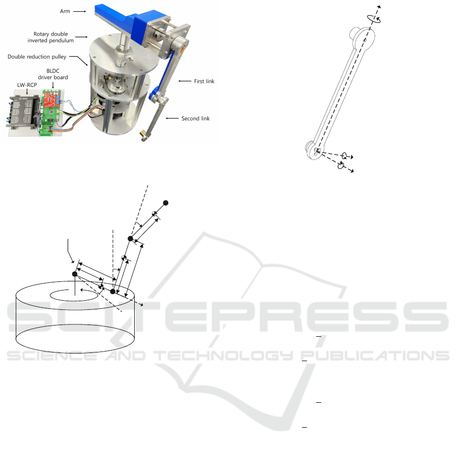
Figure 1: Rotary double inverted pendulum system con-
structed by the laboratory.
Arm
a
b
q
u
q
=
0
q
=
0
a
=
0
b
=
1
L
1
l
2
l
1
R
1
r
2
r
1
M
2
M
First link
Second link
x
1
c
2
c
Figure 2: The conceptual diagram of a rotary double in-
verted pendulum.
from the rotational axis of the first pendulum to the ro-
tational axis of the second pendulum. α is defined as
the rotational displacement of the first pendulum with
respect to the normal of the ground, and β is defined
as the relative rotational displacement of the second
pendulum with respect to the first pendulum. Addi-
tionally, c
1
and c
2
denote the friction coefficients at
the rotational axes of the first and second pendulums,
respectively. Figure 3 illustrates the rotations of the
first and second pendulums, and expressions like I
xx1
represent the moments of inertia of the pendulums(Oh
and Lee, 2018). The dynamic model of the rotary
double inverted pendulum can be derived using the
Euler-Lagrange equation and is expressed as follows.

n
1
n
2

¨
θ +

m
11
m
12
m
21
m
22

¨
α
¨
β

+

d
1
d
2

= 0. (1)
Each component of Equation (1) is defined as follows.
x
I
y
I
z
I
x
y
z
Figure 3: Rotation and inertia I of the first and second links.
n
1
= h
1
cos(α) + h
2
cos(α + β),
n
2
= h
2
cos(α + β),
m
11
= h
3
+ h
6
+ 2h
4
cos(β),
m
12
= h
6
+ h
4
cos(β),
m
21
= h
6
+ h
4
cos(β),
m
22
= h
6
,
d
1
= −h
4
sinβ(2
˙
α
˙
β +
˙
β
2
) − h
5
sinα
− h
7
sin(α + β) + c
1
˙
α
−
˙
θ
2
{
1
2
h
8
sin(2α) + h
4
sin(2α + β)
+
1
2
h
9
sin(2α + 2β)},
d
2
= h
4
sinβ(
˙
α
2
) − h
7
sin(α + β) + c
2
˙
β
−
˙
θ
2
{
1
2
h
9
sin(2α + 2β)
+
1
2
h
4
(sin(2α + 2β) − sin β)}.
h
1
to h
9
are defined as follows, and g represents the
gravitational acceleration of 9.81 [m/s
2
].
h
1
= M
1
l
1
r
1
+ M
2
L
1
(R
1
+ r
2
) − I
xz1
,
h
2
= M
2
l
2
(R
1
+ r
2
) − I
xz2
,
h
3
= I
xx1
+ M
1
l
2
1
+ M
2
L
2
1
,
h
4
= M
2
L
1
l
2
,
h
5
= g(M
1
l
1
+ M
2
L
1
),
h
6
= I
xx2
+ M
2
l
2
2
,
h
7
= M
2
gl
2
,
h
8
= M
1
l
2
1
+ M
2
L
2
1
+ I
yy1
− I
zz1
,
h
9
= M
2
l
2
2
+ I
yy2
− I
zz2
.
Thus, Equation (1) can be rearranged as follows.

¨
α
¨
β

= −

m
11
m
12
m
21
m
22

−1

n
1
n
2

¨
θ +

d
1
d
2

.
ICINCO 2024 - 21st International Conference on Informatics in Control, Automation and Robotics
94

By solving this,
¨
α =
(−m
22
n
1
+ m
12
n
2
)
¨
θ + (−m
22
d
1
+ m
12
d
2
)
Φ
,
¨
β =
(m
21
n
1
− m
11
n
2
)
¨
θ + (m
21
d
1
− m
11
d
2
)
Φ
,
Φ = m
11
m
22
− m
12
m
21
.
In this context, the state vector is defined as x
1
= θ,
x
2
= α, x
3
= β, x
4
=
˙
θ, x
5
=
˙
α, x
6
=
˙
β, x
7
=
R
t
0
θ(τ)dτ,
and the angular acceleration
¨
θ is represented as u.
Consequently, the model equation of the double in-
verted pendulum can ultimately be expressed as the
following nonlinear state equation. The last element
of the state variable,
R
t
0
θ(τ)dτ, is an additional term
introduced to eliminate the steady-state error in the
position of the arm.









˙x
1
˙x
2
˙x
3
˙x
4
˙x
5
˙x
6
˙x
7









| {z }
˙x
=










x
4
x
5
x
6
u
(−m
22
n
1
+m
12
n
2
)
¨
θ+(−m
22
d
1
+m
12
d
2
)
Φ
(m
21
n
1
−m
11
n
2
)
¨
θ+(m
21
d
1
−m
11
d
2
)
Φ
x
1










| {z }
f (x,u)
.
(2)
The dynamic model derived in this manner is subse-
quently used as the feedforward trajectory generation
model when applying the direct collocation method.
3 DESIGN AND
IMPLEMENTATION OF
TRANSITION CONTROL
3.1 Transition Control Design
The four possible equilibrium points of the rotary
double inverted pendulum, determined by the states
of the first and second pendulums, are depicted in Fig-
ure 4. In this paper, the numbering of equilibrium
points is represented using a binary notation, where
the states Up and Down are designated as 1 and 0, re-
spectively. If the numbering is assigned starting from
the first pendulum, the equilibrium point where both
the first and second pendulums are in the Down-Down
state corresponds to the binary number 00 and is de-
noted as EP0. Similarly, the equilibrium point corre-
sponding to the Up-Down state is represented by the
binary number 10 and is denoted as EP2. In this pa-
per, the equilibrium points of the inverted pendulum
will be denoted as EP0 (Down-Down), EP1 (Down-
Up), EP2 (Up-Down), and EP3 (Up-Up) according to
this method.
EP 0 EP 1 EP 2 EP 3
Figure 4: Four equilibrium points of a rotary double in-
verted pendulum.
The implemented transition control follows three
steps:
1. Linear control at the current equilibrium point.
2. Transition control from the current equilibrium
point to the next equilibrium point.
3. Linear control at the next equilibrium point.
Each transition process is structurally similar to
the swing-up problem, which involves moving the
pendulum from its initial state (EP0) to the upright
state (EP3). First, linear control is performed to en-
sure the stability of the current state before transition-
ing between the four equilibrium points. Next, tran-
sition control is executed to move from the current
equilibrium point to the next equilibrium point. Upon
reaching the new equilibrium point, additional linear
control is required to maintain stability at that point.
Thus, each transition process must satisfy both ma-
jor elements: linear control at the equilibrium points
and transition control between the equilibrium points.
Since there are a total of 12 different transition trajec-
tories for the double inverted pendulum, experiments
must be designed and conducted for each trajectory to
meet the required conditions.
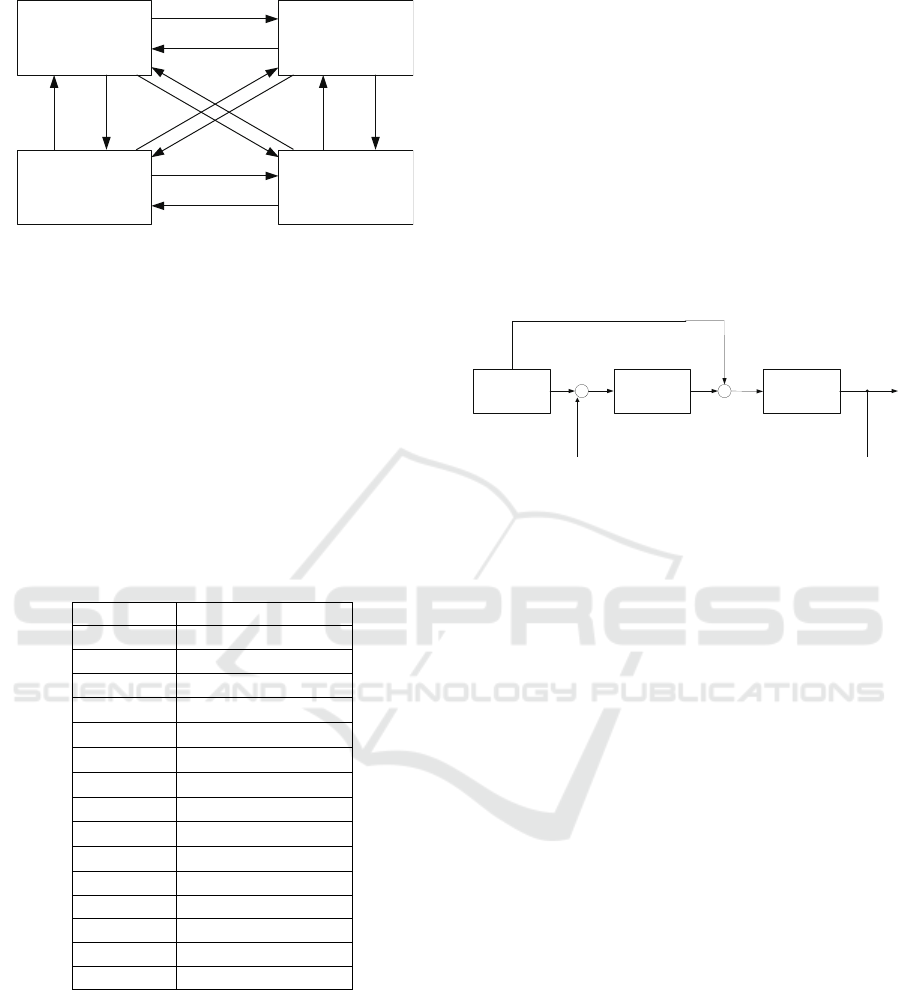
The 12 transition trajectories presented in this pa-
per are configured according to the sequence diagram
in Figure 5.
3.2 Implementation of Transition
Control
To calculate the optimal state x
∗
and control input u
∗
required for generating transition control trajectories,
Implementation of 12 Transition Controls for Rotary Double Inverted Pendulum Using Direct Collocation
95

lG
wGW
OkTP
lG
wGX
OkTP
lG
wGZ
O|TP
lG
wGY
O|TP
X
Y
Z
[
\
]
^
_
`
XW
XX
XY
Figure 5: 12-step transition diagram for the double inverted
pendulum.
it is essential to accurately estimate the parameters of
the system depicted in Figures 2 and 3. Parameters
such as M
1
, M
2
, I
xx1
, I
xx2
, l
1
, l
2
, c
1
, and c
2
can be es-
timated using the parameter estimation techniques for
the linear double inverted pendulum(Ju et al., 2022).
The estimation of the inertia tensor can be performed
by referring to the research conducted by Oh(Oh and
Lee, 2018). The parameters of the rotary double in-
verted pendulum obtained through these estimation
processes are summarized in Table 1.
Table 1: Model parameters of the rotary double inverted
pendulum used in the experiments.
Parameter Value
M
1
0.187 [kg]
M
2
0.132 [kg]
I
xx1
1.0415e-03 [kgm
2
]
I
xx2
8.8210e-04 [kgm
2
]
I
yy1
4.3569e-03 [kgm
2
]
I
yy2
4.9793e-03 [kgm
2
]
I
zz1
3.3179e-03 [kgm
2
]
I
zz2
4.8178e-03 [kgm
2
]
I
xz1
3.7770e-04 [kgm
2
]
I
xz2
1.9823e-04 [kgm
2
]
l
1
0.072 [m]
l
2
0.133 [m]
c
1
2.4100e-06
c
2
1.0900e-06
L
1
0.1645 [m]
The transition control between the equilibrium
points of the pendulum is performed using a 2-DOF
control technique that combines nonlinear feedfor-
ward control and feedback control as proposed in
(Graichen et al., 2007). Figure 6 illustrates the 2-
DOF control structure. In the control process, the pre-
computed ideal angular acceleration trajectory u
∗
(t)
is combined with the correction input ∆u(t), which
is calculated based on the error ∆x(t) = x
∗
(t) − x(t)
between the predicted state variables of the inverted
pendulum system and the actual output values. This
generates the actual angular acceleration input u(t) =
u
∗
(t)+∆u(t). In this paper, the feedforward trajectory
is generated by considering the dynamic constraints
and setting up a nonlinear optimal control problem
that numerically minimizes the desired cost function
while satisfying various constraints. The direct collo-
cation method is used to numerically solve this prob-
lem(Kelly, 2017). This method effectively estimates
the control inputs and state variable paths of contin-
uous dynamic systems and is a proven technique for
obtaining the optimal trajectory to achieve control ob-
jectives.
Signal
generator
Feedback
control
Double
Inverted
Pendulum
+
-
+
+
*
x
uD
u
*
u
x
Feedforward control
xD
Figure 6: 2-DOF control framework for the double inverted
pendulum.
The direct collocation method is an iterative nu-
merical solution implemented using a nonlinear opti-
mization solver. This method is characterized by the
influence of the initial trajectory provided by the de-
signer on the solution time of the numerical method
and the resulting trajectory’s shape. By considering
these characteristics and selecting an appropriate ini-
tial trajectory, the designer can effectively apply the
direct collocation method to derive a suitable trajec-
tory for specific transition control problems. In this
paper, the initial trajectory is designed using the sim-
plest form of a straight-line trajectory connecting the
start and end boundary conditions. Additionally, a
cost function is designed to satisfy all set constraints
and boundary conditions, forming a general nonlinear
optimal control problem. Equation (3) below repre-
sents the optimal control problem set to calculate the
optimal trajectory.
Minimize
u(t) J(x(t), u(t))
subject to input/output constraint,
dynamic equations,
boundary conditions.
(3)
In the above equation, J(x(t),u(t)) represents the
cost function and is defined as an optimal control
problem that satisfies the constraints set using the
model parameters of the actual system as listed in Ta-
ble 1. The cost function can be used either to mini-
mize time or to optimize the cost over a given period.
The constraints and limitations applied to this cost
ICINCO 2024 - 21st International Conference on Informatics in Control, Automation and Robotics
96

function include the dynamic equations of the rotary
double inverted pendulum (2) and the limits specified
by equation (4), which restrict the maximum distance
the arm can move during the control process, as well
as the maximum angular velocity and input angular
acceleration of the arm within the operational range
of the actuator. These conditions play a crucial role in
ensuring the practical operability and stability of the
control system.
|
x
∗
1
|
≤ θ
limit
,
|
x
4
∗
|
≤
˙
θ
limit
,
|
u
∗
|
≤ u
limit
.
(4)
The set limit values are all defined as positive, with
θ
limit
> 0,
˙
θlimit > 0, and ulimit > 0 specifying the
maximum allowable values for the arm’s output dis-
placement, output angular velocity, and input angular
acceleration, respectively. These limit values reflect
the actual operational constraints of the rotary double
inverted pendulum used in the experiments, and these
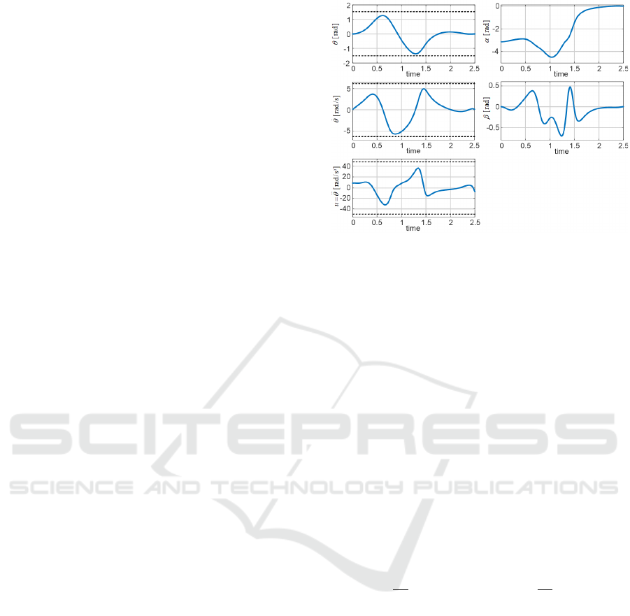
constraints are explicitly stated in equation (5).
θ
limit
= 1.5[rad],
˙
θ
limit
= 7.0[rad/s],
u
limit
= 50[rad/s
2
].
(5)
To satisfy various constraints during the 12 differ-
ent transition control processes, additional constraints
can be applied to the pendulum’s rotation angles α
and β as well as their angular velocities
˙
α and
˙
β.
Furthermore, at the start (t = 0) and end (t = T ) of
the transition control, the boundary conditions cor-
responding to the specific equilibrium points for the
transition must be satisfied. For example, if the cur-
rent equilibrium point is EP0 and the target equilib-
rium point for the transition is EP3, this situation can
be expressed as shown in equation (6).
x
∗
(0) =

0,−π,0,0, 0, 0,0

T
,
x
∗
(T ) =

0,0,0,0, 0, 0,0

T
,
u
∗
(0) = 0,u
∗
(T ) = 0.
(6)
By utilizing the direct collocation method, the transi-
tion trajectories implemented can be optimized to sat-
isfy the set constraints and boundary conditions dur-
ing the transition process, as illustrated in Figure 7.
4 EXPERIMENTAL VALIDATION
AND RESULTS
The design of the feedback controller for trajec-
tory tracking is similar to the method proposed by
Graichen(Graichen et al., 2007), mentioned in the in-
troduction. However, a key difference in this study
is the application of the optimal control technique,
Figure 7: Feedforward transition trajectory from EP0 to
EP3.
linear-quadratic (LQ) control, for time-varying sys-
tems throughout the entire process. In Graichen’s
study, it was determined that high compensation val-
ues in intervals where the gain coefficient increases
rapidly could lead to a loss of controllability, prompt-
ing the decision to suspend feedback in certain in-
tervals. In contrast, this study maintains a consis-
tent control strategy by utilizing the calculated time-
varying LQ control gain values across all intervals
during the implementation of transition control. The
design of this time-varying LQ controller is based on
the linearized dynamic system centered around the
swing-up trajectory of the double inverted pendulum
system. The state equations used in this process,
which vary with time, used in this process are mod-
eled in a form where the values of A and B are time-
varying, as shown in equation (7).
A(t) =
∂ f
∂x




x
∗
(t),u
∗
(t)
, B(t) =
∂ f
∂u




x
∗
(t),u
∗
(t)
. (7)
In this context, x
∗
(t) and u
∗
(t) represent the feed-
forward trajectories for the state and input obtained
using the direct collocation method. The difference
between the obtained feedforward trajectory and the
actual state variable values is calculated as ∆x(t) =
x
∗
(t) − x(t), and the correction input ∆u(t) generated
to compensate for this error is defined by equation (8).
∆u(t) = −K(t)∆x(t). (8)
In this case, the time-varying state equation can be
expressed as equation (9).
∆ ˙x(t) = A(t)∆x(t) + B(t)∆u(t). (9)
The cost function used is given by equation (10).
Implementation of 12 Transition Controls for Rotary Double Inverted Pendulum Using Direct Collocation
97

J = ∆x
T
(T )H
Tr
∆x(T ) +
R
T
0
∆x(t)
T
Q
Tr
∆x(t)
+∆u(t)
T
R
Tr
∆u(t)dt.
(10)
Here, the subscript Tr is used to indicate the design
variables of the transition process. In equation (10),
the variables with this subscript must satisfy H
Tr
≥ 0,
Q
Tr
≥ 0, and R
Tr
> 0. The matrix H
Tr
represents the
weight on the terminal state, the matrix Q
Tr
repre-
sents the weight on the system state, and the matrix
R
Tr
represents the weight on the control input. These
weights are set to the values of equation (11) through
an experimental process.
Q
Tr
= diag(1,300,500,1, 1, 1,1),
R
Tr
= 1.
(11)
Additionally, to calculate the time-varying gain K(t),
the differential Riccati equation presented in equation
(12) must be solved.
˙
P(t) = −A(t)
T
P(t) − P(t)A(t)
+PB(t)R
−1
Tr
B
T
(t)P(t) − Q
Tr
,
P(T ) = H
Tr
.
(12)
Ultimately, the time-varying gain K(t) can be calcu-
lated using equation (13). The LQ control gain K(t)
applied in the earlier Figure 7 can be seen in Figure 8.
K(t) = R
−1
Tr
B
T
(t)P(t). (13)
0 0.5 1 1.5 2 2.5
time(sec)
-1500
-1000
-500
0
500
1000
1500
2000
time-varying feedback gain
K
1
K
2
K
3
K
4
K
5
K
6
K
7
Figure 8: Time-varying LQ gain of feedforward transition
trajectory from EP0 to EP3.
To conduct the experiments, the swing-up trajec-
tory obtained using the direct collocation method pre-
sented in Chapter 3 is combined with the LQ control-
based feedback controller to implement the 12 differ-
ent transition controls. The trajectory paths are con-
figured according to the flowchart in Figure 5, and
the transition paths between each equilibrium point
are designed to move only once. The duration of one
cycle of state transition and linear control at the equi-
librium point is set to 5 seconds, with the time taken
for state transitions varying from a minimum of 1.8
seconds to a maximum of 3 seconds, as shown in
Table 2. After each transition, linear control is per-
formed at the corresponding equilibrium point until
the next transition control begins, to stabilize the sys-
tem. Figure 9 shows a captured image of a YouTube
video that presents the experimental results of 12 tran-
sition controls. The actual YouTube video can be ac-
cessed at https://youtu.be/J8vRJtQ-t3I (Video title: 12
transition controls of a rotary double inverted pendu-
lum (with double reduction timing pulleys), Channel
name: Embedded Control Lab.), where the experi-
mental results can be viewed in detail.
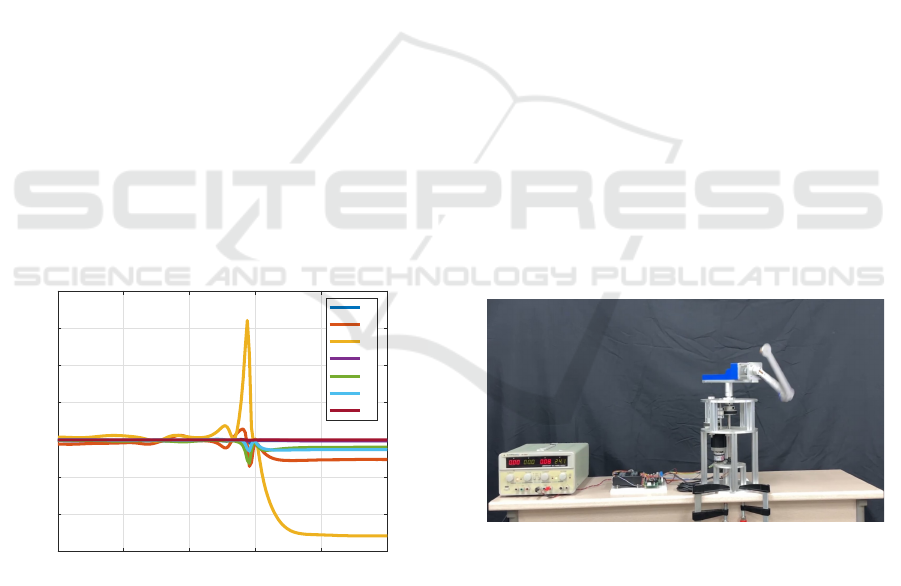
The first state transition begins at the 5-second
point, and Figure 10 shows the continuous results of
all transition controls. Each line represents the sim-
ulation model trajectory depicted by solid lines and
the actual experimental trajectory shown by dashed
lines. Due to the compensation effect of the closed-
loop control, the arm’s rotation angle θ and angular
velocity
˙
θ exhibit significant differences immediately
after the state transition, but the result graphs for α
and β, which are the most critical variables in transi-
tion control, demonstrate that the predicted paths are
followed with high accuracy. Following this, linear
control at the equilibrium point gradually adjusts the
θ value to approach zero, helping to limit the random
movement of the double pendulum and enabling all
12 transition controls to be successfully executed.
Figure 9: The Youtube video for 12 transition controls of
the RDIP.
5 CONCLUSION AND FUTURE
WORK
In this paper, we established an experimental envi-
ronment using a physically constructed rotary dou-
ble inverted pendulum system to address 12 transition
control problems, including swing-up control. We
introduced a method for generating feedforward tra-
jectories using the direct collocation technique and
ICINCO 2024 - 21st International Conference on Informatics in Control, Automation and Robotics
98

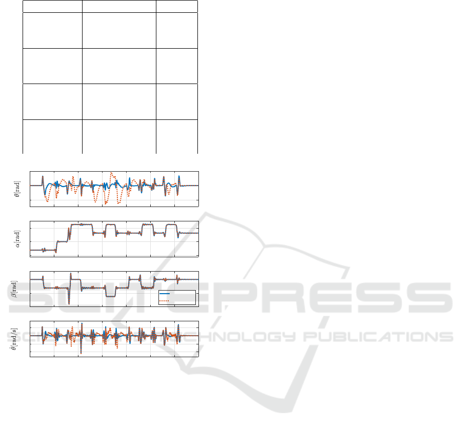
Table 2: Transition times used in the experiments.
Starting EP Destination EP T [sec]
EP0 EP1 2.000
EP2 3.000
EP3 2.500
EP1 EP0 1.800
EP2 2.500
EP3 2.500
EP2 EP0 2.500
EP1 2.000
EP3 2.921
EP3 EP0 2.500
EP1 2.000
EP2 2.000
0 10 20 30 40 50 60 70
-2
0
2
0 10 20 30 40 50 60 70
-5
0
5
0 10 20 30 40 50 60 70
-10
-5
0
simulation
true data
0 10 20 30 40 50 60 70
Time
-10
-5
0
5
Figure 10: 12-step transition trajectories of the rotary dou-
ble inverted pendulum: simulated trajectory (solid line) and
actual trajectory (dot-dashed line).
implemented these trajectories with a 2-DOF con-
troller incorporating time-varying LQ control. This
approach effectively addressed the complex transition
control problem by combining feedforward trajec-
tory generation and feedback control. The efficiency
and feasibility of the proposed method were demon-
strated through continuous control of the 12 transi-
tion paths among the four equilibrium points of the
double inverted pendulum. The main contributions
of this study include the novel definition and experi-
mental implementation of the transition control prob-
lem between equilibrium points, extending the exist-
ing swing-up problem, and the practical applicability
of the proposed control strategy validated through ex-
perimental results.
Future research can consider several directions
to further develop the transition control method pre-
sented in this paper. First, the application of a Distur-
bance Observer (DOB) technique could enhance the
robustness of the system against disturbances. Sec-
ond, incorporating artificial intelligence-based con-
trol techniques such as Reinforcement Learning could
lead to the development of more intelligent and adap-
tive control systems. Third, introducing advanced
control strategies, such as nonlinear control tech-
niques or Model Predictive Control (MPC), could be
a promising direction to improve the performance of
the controller.
As additional research, it is necessary to evaluate
the performance of the transition control under vari-
ous experimental environments and conditions to ver-
ify the generality of the proposed method. In the fu-
ture, this transition control strategy will be applied to
multi-dimensional and multi-body systems to explore
the controllability of more complex dynamic systems.
Through this, it is expected that the method can be de-
veloped into a universal control technique applicable
not only to the rotary double inverted pendulum sys-
tem but also to other complex dynamic systems.
ACKNOWLEDGEMENTS
This work was supported by the National Research
Foundation of Korea(NRF) grant funded by the Korea
government(MSIT)(RS-2024-00347193).
REFERENCES
Baek, J., Lee, C., Lee, Y. S., Jeon, S., and Han, S. (2024).
Reinforcement learning to achieve real-time control of
triple inverted pendulum. Engineering Applications of
Artificial Intelligence, 128:107518.
Brown, D. and Strube, M. (2020). Design of a neural con-
troller using reinforcement learning to control a rota-
tional inverted pendulum. In 2020 21st International
Conference on Research and Education in Mechatron-
ics (REM), pages 1–5.
¨
Astr
¨
om, K. J. and Furuta, K. (2000). Swinging up a pendu-
lum by energy control. Automatica, 36(2):287–295.
Graichen, K., Treuer, M., and Zeitz, M. (2007). Swing-up
of the double pendulum on a cart by feedforward and
feedback control with experimental validation. Auto-
matica, 43:63–71.
Ibrahim, M. M., Ubaid, M. A., Rachid, M., and Maamar,
B. (2019). Stabilization of a double inverted rotary
pendulum through fractional order integral control
scheme. International Journal of Advanced Robotic
Systems, 16(4).
Ju, D., Choi, C., Jeong, J., and Lee, Y. S. (2022). Design
and parameter estimation of a double inverted pendu-
lum for model-based swing-up control. Journal of In-
Implementation of 12 Transition Controls for Rotary Double Inverted Pendulum Using Direct Collocation
99

stitute of Control, Robotics and Systems (in Korean),
28(9):793–803.
Kelly, M. (2017). An introduction to trajectory optimiza-
tion: How to do your own direct collcation. SIAM
Review, 59(4):849–904.
Liang, F., Xin, X., and Li, Y. (2023). Swing-up and balance
control of rotary double inverted pendulum. In Pro-
ceedings of the 2023 3rd International Conference on
Robotics and Control Engineering, page 65–70.
Meta, T., Gyeong, G. Y., Park, J. H., and Lee, Y. S. (2014).
Swingup control of an inverted pendulum subject to
input/output constraints. Journal of Institute of Con-
trol, Robotics and Systems (in Korean), 20:835–841.
Oh, Y. and Lee, Y. S. (2018). Robust Swing-up Control of
a Rotary Inverted Pendulum Subject to Input/Output
Constraints. Journal of Institute of Control, Robotics
and Systems (in Korean), 24(5):423–430.
Rahairi, M., H.Selamat, Zamzuri, H., and Ahmad, F.
(2011). Pid controller optimization for a rotational
inverted pendulum using genetic algorithm. In 2011
Fourth International Conference on Modeling, Simu-
lation and Applied Optimization, pages 1–6.
Ratiroch-Anant, P., Anabuki, M., and Hirata, H. (2004).
Self-tuning control for rotational inverted pendulum
by: eigenvalue approach. In 2004 IEEE Region 10
Conference TENCON 2004., volume D, pages 542–
545.
Singh, S. and Swarup, A. (2021). Control of rotary dou-
ble inverted pendulum using sliding mode controller.
In 2021 International Conference on Intelligent Tech-
nologies (CONIT), pages 1–6.
Sondarangallage, D. A. and Manukid, P. (2019). Control of
rotary double inverted pendulum system using mixed
sensitivity h∞ controller. International Journal of Ad-
vanced Robotic Systems, 16(2).
Thein, M.-W. and Misawa, E. (1995). Comparison of the
sliding observer to several state estimators using a ro-
tational inverted pendulum. In Proceedings of 1995
34th IEEE Conference on Decision and Control, vol-
ume 4, pages 3385–3390.
Tran, N., Nguyen, V., Le, C., Lai, A., Nguyen, T., Huynh,
M., Phan, V., Tong, G., Nguyen, L., and Ngo, T.
(2024). Lqr control for experimental double rotary in-
verted pendulum. Journal of Fuzzy Systems and Con-
trol, 2(2):104–108.
Zied, B. H., Mohammad, J. F., and Zafer, B. (2020). De-
velopment of a Fuzzy-LQR and Fuzzy-LQG stabil-
ity control for a double link rotary inverted pendu-
lum. Journal of the Franklin Institute, 357(15):10529–
10556.
ICINCO 2024 - 21st International Conference on Informatics in Control, Automation and Robotics
100